|
Master Thesis Code
by Simon Moser
|
Last updated: 13. March 2024
This document is the continuation of Part 2: Kalman Filter II. Here, the Kalman filter will be extended to a RTS Smoother. The theory is based on Simon (2006), p. 293 ff., while the actual RTS Smoother is based on Rauch et al. (1965).
Until now, the filtering contained of two steps: the prediction and the update step, also called the a priori and a posteriori state estimates.
Let's introduce a new superscript notation which is also very common in the literature where
\begin{align*} \hat{x}_{k|k-1} &:= \hat{x}_{k}^{-} && \text{a priori state estimate} \\ \hat{x}_{k|k} &:= \hat{x}_{k}^{+} && \text{a posteriori state estimate}. \end{align*}
Here, a superscript - denotes the a priori state estimate and a superscript \( + \) denotes the a posteriori state estimate, e.g. \( \hat{x}_{k+10}^{-} \) is the a priori state estimate at time \( k+10 \) and \( \hat{x}_{k-10}^{+} \) is the a posteriori state estimate at time \( k-10 \) and so on.
Also, since we now do forward filtering and backward smoothing, we will use a subscript \( f \) for the forward filter and a subscript \( b \) for the backward smoother, e.g. \( \hat{x}_{f,k}^{-} \) is the forward a priori state estimate at time \( k \) and \( \hat{x}_{b,k}^{+} \) is the backward a posteriori state estimate at time \( k \) and so on.
\begin{align*} x_{k} &= F_{k}x_{k-1} + w_{k-1} \\ z_{k} &= H_{k}x_{k} + v_{k} \\ w_{k} &\sim \mathcal{N}(0, Q_{k}) \\ v_{k} &\sim \mathcal{N}(0, R_{k}). \end{align*}
\begin{align*} \hat{x}_{f,0}^+ &= \mathbb{E}[x_{0}] \\ P_{f,0}^+ &= \mathbb{E}[(x_{0} - \hat{x}_{f,0})(x_{0} - \hat{x}_{f,0})^T]. \end{align*}
\begin{align*} \hat{x}_{f,k}^- &= F_{k-1} \hat{x}_{f,k-1}^+ \\ P_{f,k}^- &= F_{k-1} P_{f,k-1}^+ F_{k-1}^T + Q_{k-1} \\[5mm] K_{f,k} &= P_{f,k}^- H_{k}^T (H_{k} P_{f,k}^- H_{k}^T + R_{k})^{-1} \\ \hat{x}_{f,k}^+ &= \hat{x}_{f,k}^- + K_{f,k}(z_{k} - H_{k} \hat{x}_{f,k}^-) \\ P_{f,k}^+ &= (I - K_{f,k} H_{k}) P_{f,k}^-. \end{align*}
\begin{align*} \hat{x}_{b,N}^+ &= \hat{x}_{f,N}^+ \\ P_{b,N}^+ &= P_{f,N}^+. \end{align*}
\begin{align*} \mathcal{I}_{f,k+1}^- &= \left(P_{f,k+1}^-\right)^{-1} \\ K_{b,k} &= P_{f,k}^+ F_{k}^T \mathcal{I}_{f,k+1}^- \\ \hat{x}_{b,k}^+ &= \hat{x}_{f,k}^+ + K_{b,k}(\hat{x}_{b,k+1}^+ - \hat{x}_{f,k+1}^-) \\ P_{b,k}^+ &= P_{f,k}^+ - K_{b,k}(P_{f,k+1}^- - P_{b,k+1}^+) K_{b,k}^T. \end{align*}
The implementation can be found in the example derivation3RtsSmoother.m.
The results of the forward filter and the backward smoother are shown in the following figure.
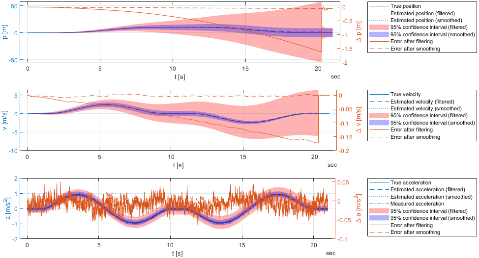
In the Image, there is only one zero-velocity update performed at the very end. Therefore, the filtered result is probably very off which is visible from the large confidence interval. The backward smoother, however, is able to correct the filtered result for the whole measurement series due to only two zero-velocity updates of the very first and very last measurement.
Also, we observe that the final confidence intervals have a constant bandwith around the estimated acceleration. This makes sense, since we're measuring acceleration. The confidence interval of the velocity, however, is larger the further the state is away from the velocity updates (i.e. the beginning and the end of the measurement series). Finally, the confidence interval of the position is constantly growing, which is also expected, since the position is the integral of the velocity and the position never gets updated.
Again, we redifine the measurement model to include position pseudo-measurements. These measurements are called pseudo-measurements since there's no actual position sensor, but we might have prior knowledge about the position at some time steps, e.g. when thinking of a TUG test, where the start and end position are at the same position (more or less) and the position of the turn around point is known (more or less), then we can use this information to correct the state estimates.
The new measurement vector is defined as follows:
\[ \mathbf{z}_k = \begin{bmatrix} z_{k,1} \\ z_{k,2} \\ z_{k,3} \end{bmatrix} = \begin{bmatrix} a_k + b_k \\ v_k \\ p_k \end{bmatrix} = \begin{bmatrix} a_\text{meas} \\ v_\text{meas} \\ p_\text{meas} \end{bmatrix}, \]
where \( a_k \) is the acceleration, \( v_k \) is the velocity, \( p_k \) is the position and \( b_k \) is the bias of the accelerometer.
The new observation matrix is therefore defined as follows:
\[ \mathbf{H}_k = \begin{bmatrix} 0 & 0 & 1 & 1 \\ 0 & 1 & 0 & 0 \\ 1 & 0 & 0 & 0\end{bmatrix}, \]
The new measurement covariance matrix is defined as follows:
\[ \mathbf{R}_k = \begin{bmatrix} 0.0449 & 0 & 0 \\ 0 & 0.001 & 0 \\ 0 & 0 & 0.5 \end{bmatrix}, \]
where 0.0449 denotes the expected deviation of the acceleration (from Allan deviation). 0.001 denotes that we are very certian about the velocity, and 0.5 denotes that we are not very certain about the position (yes, I know, this is a bit of a vague explanation). Also, in an actual application, the matrix \( \mathbf{R}_k \) would be updated to reflect the actual (pseudo-)measurement uncertainty.
Since we do not have a velocity or position information for every \( k \), the row(s) of the observation matrix are set to zero for all unavailable measurements. This leads to a Kalman gain of zero for the corresponding state vector element(s).
The implementation can be found in the example derivation3RtsSmoother.m.
The results after adding the position pseudo-measurements are shown in the following figure.
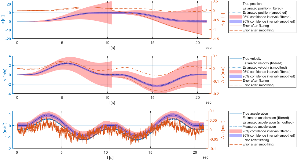
In the Image, we observe that the position pseudo-measurements are able to improve the position estimate. Also, the confidence interval of the position is now more or less a constant bandwith around the estimated position. But, when looking at the estimations of the bias \( b_k \), we observe that is changes a lot. This is due to the fact that the actual simulated sensor has a sensitivity \( s \neq 1 \) and the global optimum within the defines smoothing algorithm is achieved by changes in the bias. Therefore, we want again to supplement the state vector with the sensitivity. This leads us to a nonlinear Kalman Filter which will be discussed in the next section: Part 4: Extended Kalman Filter.