|
Master Thesis Code
by Simon Moser
|
Last updated: 14. March 2024
This document is the continuation of Part 2: Kalman Filter II and Part 3: RTS Smoother. Here, the state vector will be extended to include sensitivity.
Since the estimation of the sensitivity is nonlinear, the Kalman filter will be extended to an Extended Kalman Filter (EKF). The theory is based on Becker (2023) while the superscript notation of Simon (2006) is used.
I don't use boldface for vectors or matrices nor do I mark them in any other way that would distinguish them from scalars. This is due to the fact that I think itis simply obvious if a variable is a vector or matrix. If you don't think it is obvious, I guess this is your problem. (Not a real Quote, but close to what Dr. Franz Müller often said.)
The main idea of an EKF is to linearize the nonlinear system model and/or the nonlinear measurement model at a working point. This can be done by using a first-order Taylor expansion. The linearized models are then used in the standard Kalman filter equations.
According to Taylor's theorem a function \( f(x) \) around a working point \( x_0 \) is given by an infinite Taylor expansion (Taylor, 1717, as cited in Becker, 2023).
Also, an approximation of the nonlinear function \( f(x) \) is given with a finite first-order Taylor expansion (Becker, 2023):
\[ f(x) \approx f(x_0) + \frac{\partial f(x_0)}{\partial x} (x - x_0) \]
A Jacobian matrix is nothing else than the matrix of the first-order partial derivatives of a vector-valued function.
The state transition matrix is no longer given by the matrix \( F \) but by the nonlinear function \( f(x) \). The state transition model is then given by
\[ x_k = f\left(x_{k-1}\right) + w_k \]
where \( w_k \) is the process noise.
The state update equation is then given by
\[ \hat{x}_{f,k}^+ = f\left(\hat{x}_{f,k-1}^-\right). \]
To propagate uncertainty while keeping the gaussian PDF, the Jacobian of the state transition model is used. The Jacobian can be written as
\[ \frac{\partial f}{\partial x} \ \text {or} \ \frac{\partial f(x)}{\partial x}. \]
Then, the covariance extrapolation equation is given by
\[ P_{f,k}^- = \frac{\partial f}{\partial x} P_{f,k}^+ \left(\frac{\partial f}{\partial x}\right)^T + Q. \]
The observation model is no longer given by the matrix \( H \) but by the nonlinear function \( h(x) \). The observation model is then given by
\[ z_k = h\left(x_k\right) + v_k \]
where \( v_k \) is the measurement noise.
The state update equation is then given by
\[ \hat{x}_{f,k}^+ = \hat{x}_{f,k}^- + K_{f,k} \left(z_k - h\left(\hat{x}_{f,k}^-\right)\right). \]
To propagate uncertainty while keeping the gaussian PDF, the Jacobian of the observation model is used. The Jacobian can written as
\[ \frac{\partial h}{\partial x} \ \text {or} \ \frac{\partial h(x)}{\partial x}. \]
Then, the Kalman gain Equation is given by
\[ K_{f,k} = P_{f,k}^- \left(\frac{\partial h}{\partial x}\right)^T \left(\frac{\partial h}{\partial x} P_{f,k}^- \left(\frac{\partial h}{\partial x}\right)^T + R\right)^{-1} \]
and the covariance update equation is given by
\[ P_{f,k}^+ = \left(I - K_{f,k} \frac{\partial h}{\partial x}\right) P_{f,k}^- \left(I - K_{f,k} \frac{\partial h}{\partial x}\right)^T + K_{f,k} R K_{f,k}^T. \]
| Component | LKF | EKF | ||
|---|---|---|---|---|
| State | \( x \) | \( n \times 1 \) | \( x \) | \( n \times 1 \) |
| State Transition | \( F \) | \( n \times n \) | \( f(x) \) | \(f: \mathbb{R}^{n \times 1} \rightarrow \mathbb{R}^{n \times n} \) |
| Process Noise | \( Q \) | \( n \times n \) | \( Q \) | \( n \times n \) |
| Covariance | \( P \) | \( n \times n \) | \( P \) | \( n \times n \) |
| Observation Model | \( H \) | \( m \times n \) | \( h(x) \) | \(h: \mathbb{R}^{n \times 1} \rightarrow \mathbb{R}^{m \times n} \) |
| Measurement Noise | \( R \) | \( m \times m \) | \( R \) | \( m \times m \) |
| Kalman Gain | \( K \) | \( n \times m \) | \( K \) | \( n \times m \) |
This table is based on Becker (2023), p. 255.
| Equation | LKF | EKF | |
|---|---|---|---|
| Prediction | State extrapolation | \( \hat{x}_{f,k+1}^- = F \hat{x}_{f,k}^+ \) | \( \hat{x}_{f,k+1}^- = f\left(\hat{x}_{f,k}^+\right) \) |
| Covariance extrapolation | \( P_{f,k+1}^- = F P_{f,k}^+ F^T + Q \) | \( P_{f,k+1}^- = \frac{\partial f}{\partial x} P_{f,k}^+ \left(\frac{\partial f}{\partial x}\right)^T + Q \) | |
| Update | Kalman gain | \begin{align*} K_{f,k} &= P_{f,k}^- H^T \\ &\times \left(H P_{f,k}^- H^T + R\right)^{-1} \end{align*} | \begin{align*} K_{f,k} &= P_{f,k}^- \left(\frac{\partial h}{\partial x}\right)^T \\ &\times \left(\frac{\partial h}{\partial x} P_{f,k}^- \left(\frac{\partial h}{\partial x}\right)^T + R\right)^{-1} \end{align*} |
| State update | \( \hat{x}_{f,k}^+ = \hat{x}_{f,k}^- + K_{f,k} \left(z_k - H \hat{x}_{f,k}^-\right) \) | \( \hat{x}_{f,k}^+ = \hat{x}_{f,k}^- + K_{f,k} \left(z_k - h\left(\hat{x}_{f,k}^-\right)\right) \) | |
| Covariance update | \begin{align*} P_{f,k}^+ &= \left(I - K_{f,k} H\right) P_{f,k}^- \\ &\times \left(I - K_{f,k} H\right)^T + K_{f,k} R K_{f,k}^T \end{align*} | \begin{align*} P_{f,k}^+ &= \left(I - K_{f,k} \frac{\partial h}{\partial x}\right) P_{f,k}^- \\ &\times \left(I - K_{f,k} \frac{\partial h}{\partial x}\right)^T + K_{f,k} R K_{f,k}^T \end{align*} |
Now, the previously used single-axis movement estimation will be extended to include sensitivity.
The new state vector is given by
\[ x = \begin{bmatrix} p \\ v \\ a \\ b \\ s \end{bmatrix}, \]
where \( p \) is the position, \( v \) is the velocity, \( a \) is the acceleration of the object and \( b \) and \( s \) are the bias and sensitivity of the accelerometer, respectively.
The state transition model remains linear and is given by
\[ f(x) = F = \begin{bmatrix} 1 & \Delta t & \frac{1}{2} \Delta t^2 & 0 & 0 \\ 0 & 1 & \Delta t & 0 & 0 \\ 0 & 0 & 1 & 0 & 0 \\ 0 & 0 & 0 & 1 & 0 \\ 0 & 0 & 0 & 0 & 1 \end{bmatrix}. \]
Therefore, there is no need to linearize the state transition model.
The initial state is given by
\[ x_0 = \begin{bmatrix} 0 \\ 0 \\ 0 \\ 0 \\ 1 \end{bmatrix}. \]
The covariance estimate covariance is identical to an LKF given by
\[ P = \begin{bmatrix} \sigma_p^2 & \sigma_{pv} & \sigma_{pa} & \sigma_{pb} & \sigma_{ps} \\ \sigma_{pv} & \sigma_v^2 & \sigma_{va} & \sigma_{vb} & \sigma_{vs} \\ \sigma_{pa} & \sigma_{va} & \sigma_a^2 & \sigma_{ab} & \sigma_{as} \\ \sigma_{pb} & \sigma_{vb} & \sigma_{ab} & \sigma_b^2 & \sigma_{bs} \\ \sigma_{ps} & \sigma_{vs} & \sigma_{as} & \sigma_{bs} & \sigma_s^2 \end{bmatrix}. \]
The a priori estimate of the initial covariance is given by
\[ P_0 = \begin{bmatrix} 0 & 0 & 0 & 0 & 0 \\ 0 & 0 & 0 & 0 & 0 \\ 0 & 0 & 0 & 0 & 0 \\ 0 & 0 & 0 & 0.59^2 & 0 \\ 0 & 0 & 0 & 0 & 0.03^2 \end{bmatrix}, \]
where the position and velocity are assumed to be known perfectly. According to the datasheet, the accelerometer has a bias which es expected to be normally distributed around \( 0 \) with a standard deviation of \( 0.59 \ \mathrm{\frac{m}{s^2}} \). The sensitivity is expected to be normally distributed around \( 1 \) with a standard deviation of \( 3 \% \).
The process noise is identical to an LKF and given by
\[ Q = \begin{bmatrix} \frac{\Delta t^4}{4} & \frac{\Delta t^3}{2} & \frac{\Delta t^2}{2} & 0 & 0 \\ \frac{\Delta t^3}{2} & \Delta t^2 & \Delta t & 0 & 0 \\ \frac{\Delta t^2}{2} & \Delta t & 1 & 0 & 0 \\ 0 & 0 & 0 & 0 & 0 \\ 0 & 0 & 0 & 0 & 0 \end{bmatrix} \sigma_a^2, \]
where \( \sigma_a^2 \) is set to \( 0.0025 \ \mathrm{\frac{m^2}{s^4}} \). The process noise of the bias and sensitivity is assumed to be zero.
The measurement vector is given by
\[ z = \begin{bmatrix} p_{\text{meas}} \\ v_{\text{meas}} \\ a_{\text{meas}} \end{bmatrix} = \begin{bmatrix} p \\ v \\ a \cdot s + b \end{bmatrix}. \]
This means that the measurements of the position and velocity are identical to the actual state. This obviously holds only in our case, where we have pseudo-measurements. The acceleration measurement model is close to a real-world accelerometer, while still ignoring temperature and other influences.
The Jacobian is given by
\begin{align*} \frac{\partial h}{\partial x} &= \begin{bmatrix} \frac{\partial h_1}{\partial x_1} & \cdots & \frac{\partial h_1}{\partial x_n} \\ \vdots & \ddots & \vdots \\ \frac{\partial h_m}{\partial x_1} & \cdots & \frac{\partial h_m}{\partial x_n} \end{bmatrix} \\[3mm] &= \begin{bmatrix} \frac{\partial (p)}{\partial (p)} & \frac{\partial (p)}{\partial (v)} & \frac{\partial (p)}{\partial (a)} & \frac{\partial (p)}{\partial (b)} & \frac{\partial (p)}{\partial (s)} \\ \frac{\partial (v)}{\partial (p)} & \frac{\partial (v)}{\partial (v)} & \frac{\partial (v)}{\partial (a)} & \frac{\partial (v)}{\partial (b)} & \frac{\partial (v)}{\partial (s)} \\ \frac{\partial (a \cdot s + b)}{\partial (p)} & \frac{\partial (a \cdot s + b)}{\partial (v)} & \frac{\partial (a \cdot s + b)}{\partial (a)} & \frac{\partial (a \cdot s + b)}{\partial (b)} & \frac{\partial (a \cdot s + b)}{\partial (s)} \end{bmatrix} \\[3mm] &= \begin{bmatrix} 1 & 0 & 0 & 0 & 0 \\ 0 & 1 & 0 & 0 & 0 \\ 0 & 0 & s & 1 & a \end{bmatrix}. \end{align*}
The measurement uncertainty is identical to a LKF and is given by
\[ R_k = \begin{bmatrix} \sigma_{p_{\text{pseudo}_k}} & 0 & 0 \\ 0 & \sigma_{v_{\text{pseudo}_k}} & 0 \\ 0 & 0 & \sigma_a^2 \end{bmatrix}, \]
where \( \sigma_{p_{\text{pseudo}_k}} \) and \( \sigma_{v_{\text{pseudo}_k}} \) are set accordingly to reflect the certainty of the pseudo-measurements. The acceleration measurement is assumed to be normally distributed around \( 0 \) with a standard deviation of \( 0.0449 \ \mathrm{\frac{m}{s^2}} \) (result from Allan Deviation Experiments).
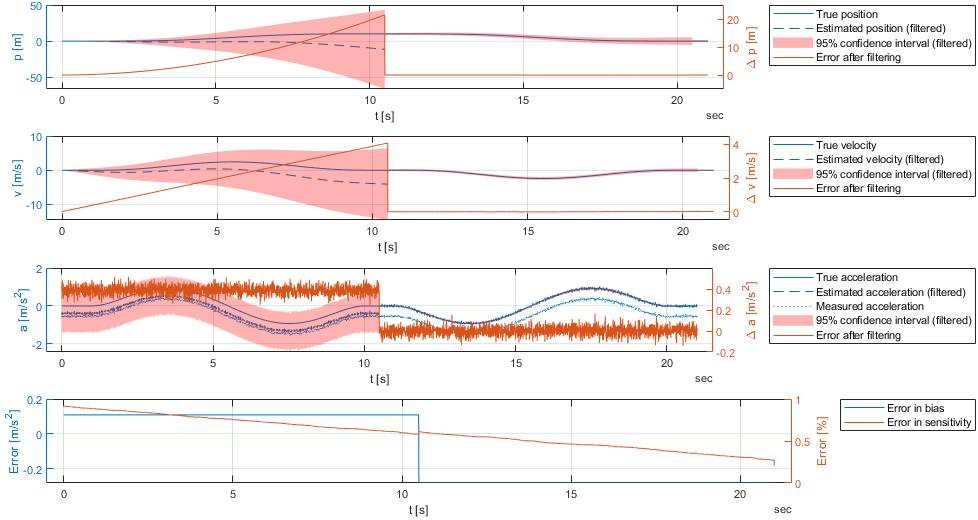
A working example can be found in the example derivation4ExtendedKalmanFilter.m. The following code is a simplified version of the example.
The results of the filtering can be seen in the following figure. The position, velocity, and acceleration are shown in the first three subplots. The bias and sensitivity errors are shown in the last subplot.
Since our extrapolation model is linear, the RTS smoother equations are identical to the LKF and are given by
\begin{align*} \mathcal{I}_{f,k+1}^- &= \left(P_{f,k+1}^-\right)^{-1} \\ K_{b,k} &= P_{f,k}^+ F^T \mathcal{I}_{f,k+1}^- \\ \hat{x}_{b,k}^+ &= \hat{x}_{f,k}^+ + K_{b,k}(\hat{x}_{b,k+1}^+ - \hat{x}_{f,k+1}^-) \\ P_{b,k}^+ &= P_{f,k}^+ - K_{b,k}(P_{f,k+1}^- - P_{b,k+1}^+) K_{b,k}^T. \end{align*}
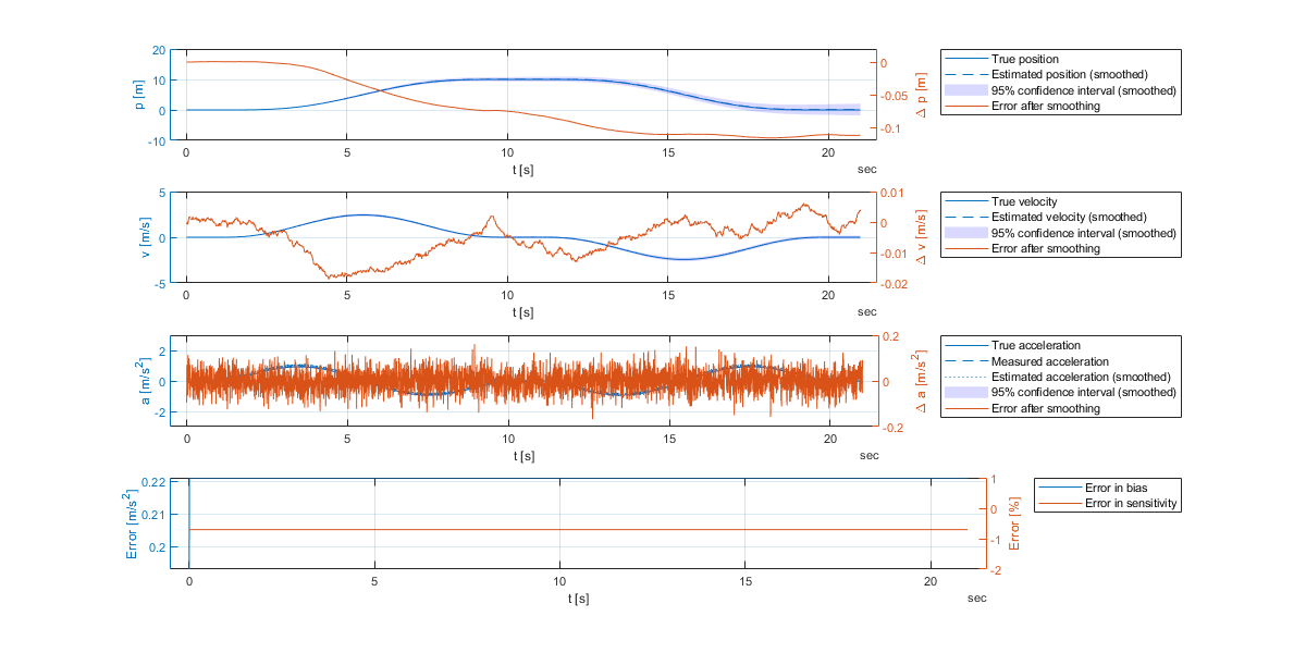
A working example can be found in the example derivation4ExtendedKalmanFilter.m. The following code is a simplified version of the example.
_fp, _fm, and _bp are used to distinguish between the a priori, a posteriori, and a posteriori smoothed estimates, respectively.The results of the smoothing can be seen in the following figure. The position, velocity, and acceleration are shown in the first three subplots. The bias and sensitivity errors are shown in the last subplot.
The Extended Kalman Filter (EKF) was derived and applied to a single-axis movement estimation. The results show that the EKF is able to estimate the bias and sensitivity of the accelerometer. However, an EKF with a sensitivity performed worse than a LKF without sensitivity in our tests. But, if smoothing, the EKF-RTS approach performed a bit better than the LKF-RTS approach.