|
Master Thesis Code
by Simon Moser
|
Last updated: 29. April 2024
As we have seen in Part 6: 6D EKF-RTS we're struggeling with wrong estimations of biases and sensitivities. Therefore sifferent approaches to mitigate these issues are presented in this part.
The first approach is to use the same EKF architecture as in Part 6: 6D EKF-RTS but with different initial values. The initial values for the accelerometer biases and sensitivies are calculated using the algorithm presented in derivation7InitialParamEst. Since then the initial values are more accurate, the initial covariance matrix is set to a smaller value. The implementation of this approach can be found in derivation8Ekf6D_pt1.m.
When setting the flag USE_REAL_DATA, the algorithm is run with the real data. If not, the algorithm is run with the simulated data. The results of the algorithm are shown in the following section.
The state of implementation including the tuning parameters can be found in this commit.
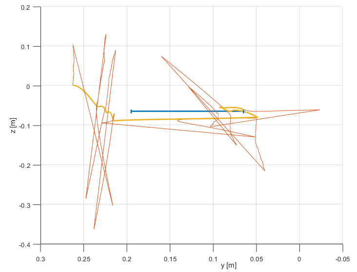
In the following plots, the real position is blue, the estimation based on the filter is orange, and the smoothed position estimation is yellow.
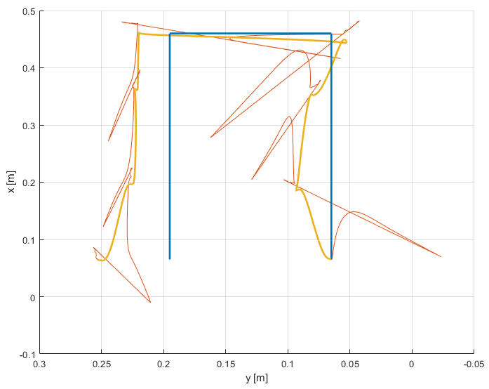
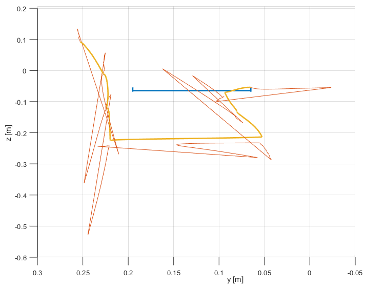
It's visible that the position estimations of the forward pass tend to diverge from the real position which happens when no zero-velocity (ZV) is detected. As soon as the next ZV range is detected, the position 'jumps' back close to the real position. Therefore, the position estimations of the backward pass are more accurate than the forward pass. The smooting result and even the final position of the filter is in a very acceptable range considering the fact that everything is based on IMU data only and no additional information was applied (e.g. height reset during ZV, final position pseudo-measurement, etc.). But clearly, the position estimations are not as accurate as they should be and also the spikes in the filteres results must be mitigated.
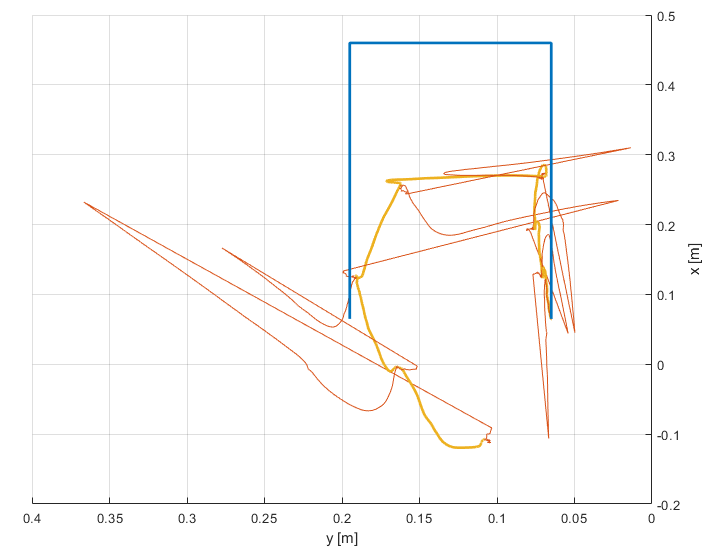
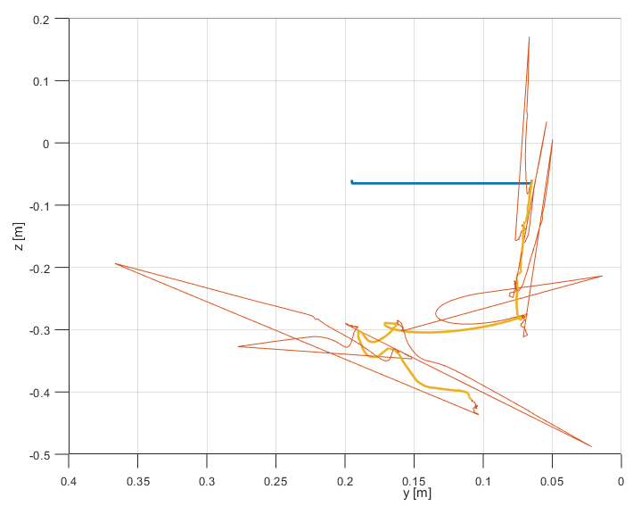
The results of the real data are less accurate than the simulated data. But again, the position estimation does not diverge too much from the real position which is considered as a good result. The spikes in the filteres results are also visible in the real data. The position estimations of the backward pass are more accurate than the forward pass. It is assumed that the difference between the simulated and real data is due to the fact that such homogeneous movements as in the simulation are not present when I move things around in the real world.
The results of this approach are not satisfying. The position estimations are not as accurate as they should be and the spikes in the filteres results must be mitigated. Therefore, a different approach is presented in the next section.
Since it is assumed that the key of this whole work is the clever introduction of pseudo-measurements, the next approach is to introduce a pseudo-measurement for the position. This approach is presented in the next section.
The second approach is to introduce a pseudo-measurement for the position. One obvious choice for the pseudo-measurement is the z-coordinate of the position during ZV. The implementation of this approach can be found in derivation8Ekf6D_pt2.m.
To enable position pseudo-measurements, the measurement model must be updated. The derived model from Part 6: 6D EKF-RTS is extended by the position pseudo-measurement. The extension is straight forward and given by
\begin{align*} \mathbf{h}_4(\mathbf{x}) &= \mathbf{p} \end{align*}
with the jacobian
\begin{align*} \mathbf{H}_4 &= \begin{bmatrix} \mathbf{0}_{3 \times 10} & \mathbf{I}_3 & \mathbf{0}_{3 \times 12} \end{bmatrix} \end{align*}
where \(\mathbf{p}\) is the 'known' position.
Also, the measurement noise covariance matrix \(\mathbf{R}\) must be extended with appropriate values for the position pseudo-measurement.
The first implemented position pseudo-measurement is the z-coordinate of the position during ZV. We know that the true z-coordinate of the position is in the range \( [-0.06,0.07] \) m. Therefore a pseudo-measurement of \( \mathbf{p} = \begin{bmatrix}0&0&-0.065\end{bmatrix}^T \) m is introduced during ZV. The measurement noise covariance matrix is then set to
\[ \mathbf{R}_\text{new} = \begin{bmatrix} \mathbf{R}_\text{old} && & \mathbf{0} \\ & \infty \\ & & \infty \\ \mathbf{0} & & & \sigma_\text{pseudo}^\text{(pos)} \end{bmatrix}, \]
where \(\mathbf{R}_\text{old}\) is the measurement noise covariance matrix of the derived model from Part 6: 6D EKF-RTS and \(\sigma_\text{pseudo}^\text{(pos)}\) is the variance of the pseudo-measurement. The infinite values lead to zero Kalman gain for the \( x\) and \( y\) coordinates during ZV. Another method is to set the corresponsing rows of the \(\mathbf{H}\) matrix to zero. This also leads to zero Kalman gain for the \( x\) and \( y\) coordinates during ZV.
While testing different values, a variance of \( \sigma_\text{pseudo}^\text{(pos)} = 0.05 \) m was found to be a good value. All other parameters were kept the same as in the previous approach.
In the following plots, the real position is blue, the estimation based on the filter is orange, and the smoothed position estimation is yellow.
The state of the implementation including the tuning parameters can be found in this commit.
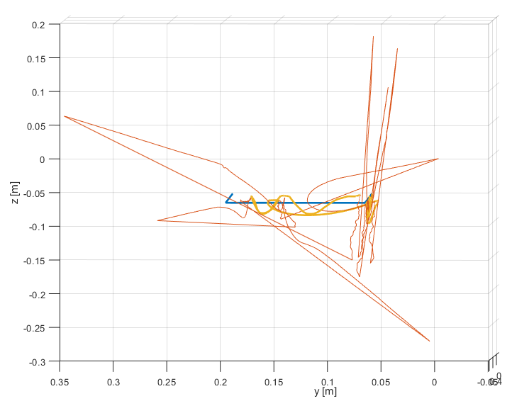
The top view looks similar to the previous approach, therefore only the front view is shown.
Clearly the errors in z-direction are minimized by the pseudo-measurement. An actual correction of any other state based on correlation didn't happen.
The top view looks similar to the previous approach, therefore only the front view is shown.
Also in the real data, the errors in z-direction are minimized by the pseudo-measurement, but this didn't lead to a better estimation of the position on the xy-plane.
Now, also one final pseudo-measurement is introduced at the end of the dataset. This means that
\begin{align*} \mathbf{z}_{{(13:15)}_{N-100:N}} = \begin{bmatrix} 0.065 & 0.195 & -0.06 \end{bmatrix}^T \end{align*}
and all three entries of the measurement noise covariance matrix are set to \( \sigma_\text{pseudo}^\text{(pos)} = 0.05 \) m for the final one hundred samples.
The state of the implementation including the tuning parameters can be found in this commit.
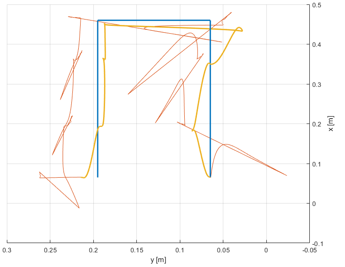
At the end of the filtered trajectory the movement towards the set final position is clearly visible. Since the backward pass starts at the final filter state, the position "measurement" develops its full effect in the backward pass. The smoothed position estimations are very close to the ground truth.
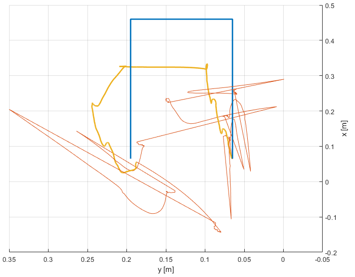
Again, the results of the real data are less accurate than the simulated data. But the movement towards the set final position is also visible in the real data. The smoothed position estimations are a lot better than the results without the final pseudo-measurement.
The results indicate the importance of the pseudo-measurement for the position. The errors in z-direction are minimized by the pseudo-measurement. Actual position pseudo-measurements are a very powerful tool to improve the position estimation. But what is still missing is the mitigation of the spikes in the filteres results. Therefore, a different approach is presented in the next section. It is assumed that the spikes are due to the prediction of the angular velocity. Since a constant angular velocity is assumed, at a start of a rotation the prediction would still assume the constant, i.e. zero, angular velocity. This leads to a lag of the estimated angular velocity. Therefore, the next approach is to move the angular velocity to the control input. This approach is presented in the next part: Part 9: 6D EKF-RTS.
As a final test of the algorithm, the filtering and smoothing of an actual walking trajectory is performed.
The measurement comes from a walking task that consists of
The filter is runned with different kinds of pseudo-measurements of the position:
The results are shown below. Besides the added pseudo-measurements, the filter is runned with the same parameters for all approaches. The implementation of this approach can be found in derivation8Ekf6D_pt3.m.
The state of the implementation can be found in this commit.
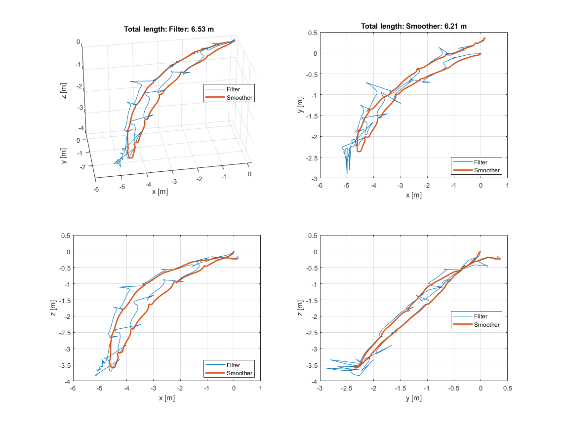
Even tough the algorithm knew nothing about the final position, the final position is only about 0.45 m off the real position. The estimated total length of the trajectory is estimated to be 6.53 m and 6.21 m for the filter and smoother, respectively. The real length of the trajectory is 9 m. Also, some bias in the z-direction is visible leading to a z-position of up to 3.5 m above ground.
The state of the implementation can be found in this commit.
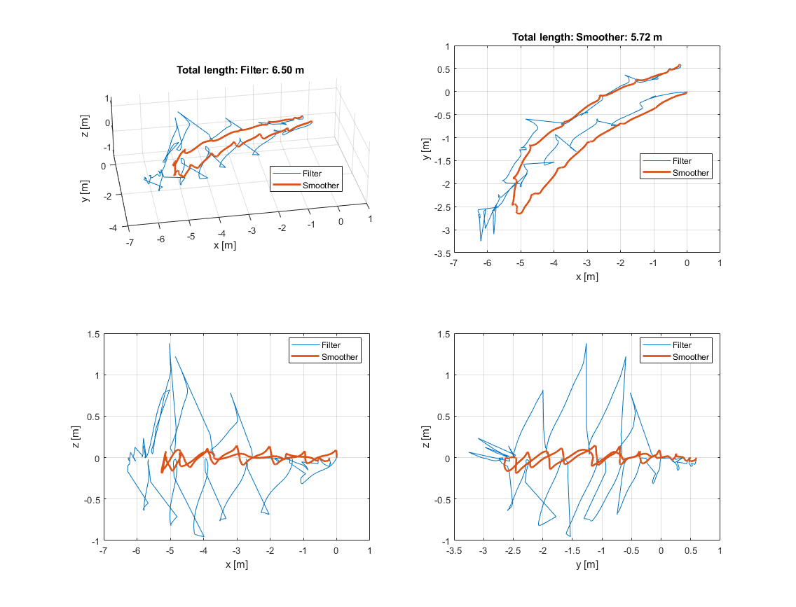
The z-position is now very close to the ground. The estimated total length of the trajectory is estimated to be 6.5 m and 5.72 m for the filter and smoother, respectively. The final position is about 0.64 m off the real position. Positive z-values are still present, even though they are impossible because of the floor. It is assumed that the positive z-values are due to the fact that we assume constant acceleration and that this model is not able to capture the acceleration change during the beginning of the stance phase.
The state of the implementation can be found in this commit.
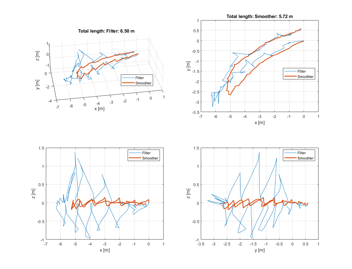
As expected, this change doesn't havve a significant effect on the position estimation. The estimated total length of the trajectory is estimated to be 6.5 m and 5.72 m for the filter and smoother, respectively. The final position is about 0.63 m off the real position. Positive z-values are still present, even though they are impossible because of the floor.
The state of the implementation can be found in this commit.
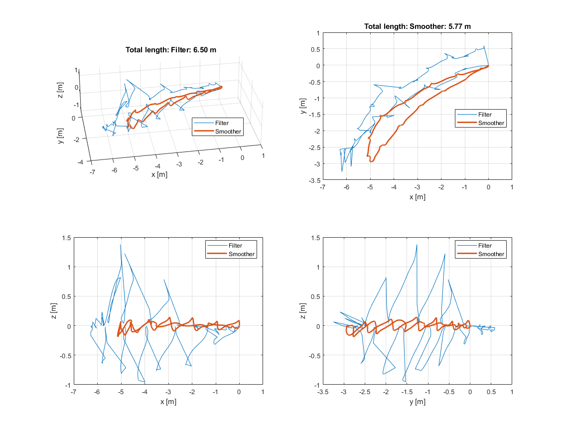
Now, the final position is only about 1 cm off the real position which is maybe even closer to the initial position than the final position was in real. The estimated total length of the trajectory is estimated to be 6.5 m and 5.77 m for the filter and smoother, respectively. Positive z-values are still present.
The state of the implementation can be found in this commit.
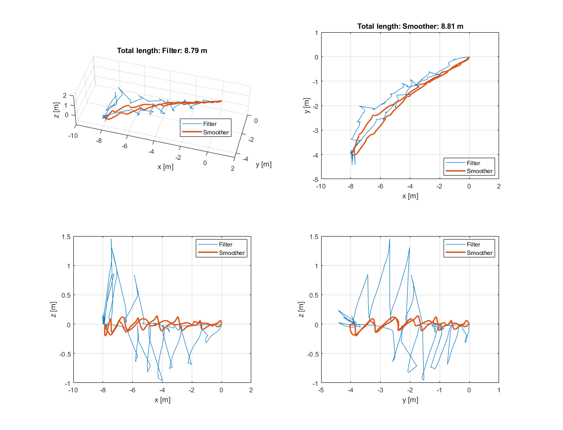
The estimated total length of the trajectory is estimated to be 8.79 m and 8.81 m for the filter and smoother, respectively. The final position is about 0.01 m off the real position. Positive z-values are still present. The strength of the pseudo-measurement in the turning phase becomes clearly visible.
Even tough all this sounds very promising, when looking at the estimated biases and sensitivities, the results are not satisfying. The estimated biases and sensitivities are still far off the (likely) real values as you can see in the following plot. The estimated values are shown in blue, orange, and yellow for the x,y, and z-axis, respectively (smoother). The estimated values from the 6-faces calibration are shown in black.
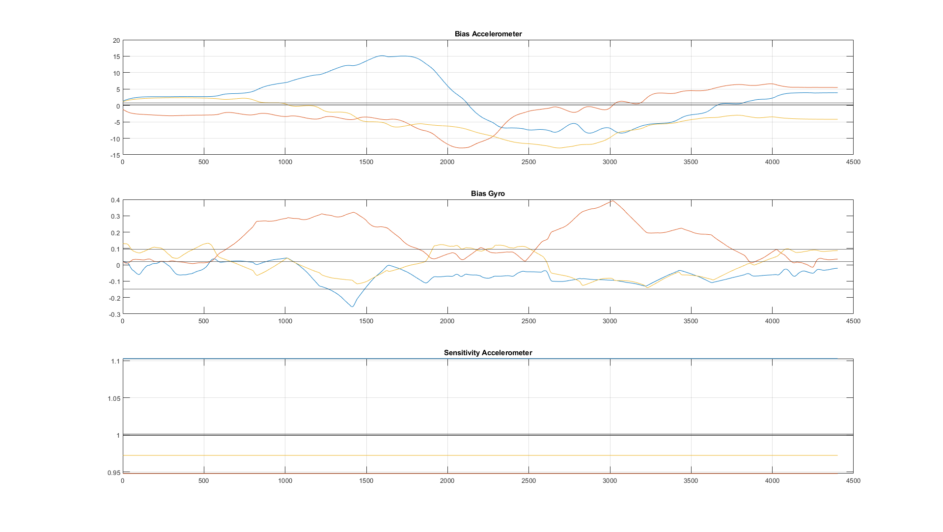
It's very positive that the same filter did work and not diverge also for data of a walkong trajectory. However, the limitations in the prediction models become more and more visible. The estimated biases and sensitivities are still far off the (likely) real values. Therefore, a different approach is presented in the next part: Part 9: 6D EKF-RTS