|
Master Thesis Code
by Simon Moser
|
Last updated: 4. April 2024
In this and the following documents a first relatively simple six dimensional EKF-RTS is derived to make a sensor fusion of a 3-axis accelerometer and a 3-axis gyroscope to estimate the 3D position and orientation. The EKF-RTS is first tested on simulated data from the JumpSensor and then on real data.
The movement is just the sensor mounted in the cube holder and then turned in such a way that every face of the cube is facing down at least once. The real movement where the sensor is mounted in the cube holder and the corresponding simulated movement is shown in the following animation.
In this document, we'll only consider the orientation estimation. The position estimation will be considered in the next document. Therefore we use simulated data from the above mentioned movement but we set all positions to zero before simulating.
As we've seen in the last parts of this series, we obtain the position of our sensor by integrating the acceleration twice. Also we've seen, that even small biases in the acceleration measurement lead to huge errors due to the double integration. When dealing with a three dimensional sensor, we also have to consider the orientation of the sensor. Again, we are not able to measure the absolute orientation, bot only angular velocities. We need a very accurate estimate of the orientation because we have to subtract the gravity from the acceleration before we integrate. As already Rutishauser (2014, p. 24) showed, a wrong orientation estimate of only 1° leads to an error of close to 10 cm in the horizontal plane, per second.
Parts of the background are inspired by this site and Rutishauser (2014).
Since we start to rotate the sensor, there exists a local coordinate system of the sensor and a global coordinate system. In the notation the coordinate system is represented by a preceding superscript. The local coordinate system of the sensor is denoted by \( s \) and the global coordinate system is denoted by \( g \). The local coordinate system of the sensor is also called the sensor frame and the global coordinate system is also called the world frame.
There are several ways to represent orientation. The most common are Euler angles, rotation matrices, quaternions and modified Rodrigues parameters. Euler angles are the most intuitive, but they suffer from gimbal lock and can be ambiguously defined. Rotation matrices aren't ambiguous, but they have 9 parameters. Both quaternions and modified Rodrigues parameters are unambiguous. Quaternions have 4 parameters and modified Rodrigues parameters have 3 parameters. There are different opinions on which representation is the best. While quaternions can be a bit unintuitive at first, they are assumed to be more computationally efficient, are numerically stabler and are most commonly used in the literature and software libraries. Therefore, we will use quaternions to represent the orientation. (Honestly, I just decided to use quaternions some months ago and also implemented them in the code. I didn't do a thorough comparison of the different representations and now I just want to stick with quaternions.)
Quaternion orientation is described as a rotation angle \( \alpha \) around an euler axis \( e = (e_1, e_2, e_3) \). The quaternion is then defined as
\[ q = \begin{bmatrix} q_0 \\ q_1 \\ q_2 \\ q_3 \end{bmatrix} = \begin{bmatrix} \cos \alpha \\ e_1 \sin \left( \frac{\alpha}{2} \right) \\ e_2 \sin \left( \frac{\alpha}{2} \right) \\ e_3 \sin \left( \frac{\alpha}{2} \right) \end{bmatrix}. \]
The quaternion kinematic differential equation is given by
\[ \dot{q} = \frac{1}{2} \begin{bmatrix} -q_1 & -q_2 & -q_3 \\ q_0 & -q_3 & q_2 \\ q_3 & q_0 & -q_1 \\ -q_2 & q_1 & q_0 \end{bmatrix} \begin{bmatrix} \prescript{s}{}{\omega_x} \\ \prescript{s}{}{\omega_y} \\ \prescript{s}{}{\omega_z} \end{bmatrix} \]
where \( \prescript{s}{}{\omega} \) is the angular velocity in the sensor frame (Diebel, 2006).
Following the explanations here which are based on Wertz (1978), the discrete time update of the quaternion is given by
\[ q_{k+1} = \left[ \cos \left( \frac{||\prescript{s}{}{\omega}|| \Delta t}{2}\right) I_4 + \frac{1}{||\prescript{s}{}{\omega}||} \sin \left( \frac{||\prescript{s}{}{\omega}|| \Delta t}{2} \right) \Omega(\prescript{s}{}{\omega}) \right] q_k, \]
where \( I_4 \) is the 4x4 identity matrix, and \( \Omega(\prescript{s}{}{\omega}) \) is an operator matrix defined by
\[ \Omega(\prescript{s}{}{\omega}) = \begin{bmatrix} 0 & -\prescript{s}{}{\omega}^T \\ \prescript{s}{}{\omega} & - \lfloor \prescript{s}{}{\omega} \rfloor_{\times} \end{bmatrix} = \begin{bmatrix} 0 & -\prescript{s}{}{\omega_x} & -\prescript{s}{}{\omega_y} & -\prescript{s}{}{\omega_z} \\ \prescript{s}{}{\omega_x} & 0 & \prescript{s}{}{\omega_z} & -\prescript{s}{}{\omega_y} \\ \prescript{s}{}{\omega_y} & -\prescript{s}{}{\omega_z} & 0 & \prescript{s}{}{\omega_x} \\ \prescript{s}{}{\omega_z} & \prescript{s}{}{\omega_y} & -\prescript{s}{}{\omega_x} & 0 \end{bmatrix}, \]
where the operator \( \lfloor \prescript{s}{}{\omega} \rfloor_{\times} \) expands the 3x1 vector \( \prescript{s}{}{\omega} \) to a 3x3 skew-symmetric matrix.
The first order Taylor approximation of the discrete quaternion kinematic differential equation is given by
\[ q_{k+1} \approx \left[ I_4 + \frac{1}{2}\Omega(\prescript{s}{}{\omega}) \Delta t \right] q_k. \]
THis can also be written with quaternion multiplication as
\[ q_{k+1} \approx q_k \otimes \left[ 1 + \frac{1}{2} \prescript{s}{}{\omega} \Delta t \right], \]
where \( \otimes \) denotes the quaternion multiplication (Solà, 2017).
Since this is an approximation, the quaternion has to be normalized after each update:
\[ q_{k+1} \leftarrow \frac{q_{k+1}}{||q_{k+1}||}. \]
The roll and pitch angles can be calculated from the accelerometer measurements. The roll angle is given by
\[ \phi = \arctan \left( \frac{a_y}{a_z} \right) \]
and the pitch angle is given by
\[ \theta = \arcsin \left( \frac{a_x}{\sqrt{a_x^2 + a_y^2 + a_z^2}} \right). \]
The state vector is given by
\[ x = \begin{bmatrix} q \\ \omega \\ b_{\text{gyr}} \\ b_{\text{acc}} \\ s_{\text{gyr}} \\ s_{\text{acc}} \\ \end{bmatrix}, \]
where \( q \in \mathbb{R}^{4\times 1} \) are the four quaternion components, \( \omega \in \mathbb{R}^{3\times 1} \) is the angular velocity \( b_{\text{gyr}} \in \mathbb{R}^{3\times 1} \) is the gyroscope bias, \( b_{\text{acc}} \in \mathbb{R}^{3\times 1} \) is the accelerometer bias, \( s_{\text{gyr}} \in \mathbb{R}^{3\times 1} \) is the gyroscope scale factor and \( s_{\text{acc}} \in \mathbb{R}^{3\times 1} \) is the accelerometer scale factor which leads to \( x \in \mathbb{R}^{19\times 1} \).
We assume that we know the initial orientation, that biases are zero and the scale factors are one. Therefore, the initial state is given by
\[ x_0 = \begin{bmatrix} 1 \\ \mathbf{0}_{12 \times 1} \\ \mathbf{1}_{6 \times 1} \end{bmatrix}. \]
In this section, we derive the state extrapolation model for the orientation. We assume a constant angular velocity and constant biases and sensitivity.
To keep the notation simple, the state transition function is split into \( n \) independant parts. The complete state transition function is then given by
\[ f = \begin{bmatrix} f_1 \\ f_2 \\ f_3 \\ \end{bmatrix}, \]
where \( f_i \) is the \( i \)-th part of the state transition function.
Similarly, the Jacobian of the state transition function is given by
\[ F_k = \begin{bmatrix} F_1 & \mathbf{0}_{4 \times 12} \\ \mathbf{0}_{15 \times 4} & F_2 \oplus F_3 \oplus F_4 \oplus F_5 \oplus F_6 \end{bmatrix}, \]
where \( F_i \) is the Jacobian of the \( i \)-th part of the state transition function and \( \oplus \) denotes the direct sum.
From the above equations, the state extrapolation model for the orientation is given by
\[ \hat{q}_{k+1}^- = \left[ I_4 + \frac{1}{2}\Omega(\prescript{s}{}{\hat{\omega}_k^+}) \Delta t \right] \hat{q}_k^+, \]
assuming a constant angular velocity.
The quaternion extrapolation is given by the quaternion extrapolation equation
\begin{align*} \hat{q}_{k+1}^- &= f_1(\hat{\omega}_k^+, \hat{q}_k^+) \\[3mm] &= \left[ I_4 + \frac{1}{2}\Omega(\prescript{s}{}{\hat{\omega}_k^+}) \Delta t \right] \hat{q}_k^+ \\[3mm] &= \begin{bmatrix} \frac{2}{\Delta t} & -\prescript{s}{}{\hat{\omega}_{x_k}^+} & -\prescript{s}{}{\hat{\omega}_{y_k}^+} & -\prescript{s}{}{\hat{\omega}_{z_k}^+} \\ \prescript{s}{}{\hat{\omega}_{x_k}^+} & \frac{2}{\Delta t} & \prescript{s}{}{\hat{\omega}_{z_k}^+} & -\prescript{s}{}{\hat{\omega}_{y_k}^+} \\ \prescript{s}{}{\hat{\omega}_{y_k}^+} & -\prescript{s}{}{\hat{\omega}_{z_k}^+} & \frac{2}{\Delta t} & \prescript{s}{}{\hat{\omega}_{x_k}^+} \\ \prescript{s}{}{\hat{\omega}_{z_k}^+} & \prescript{s}{}{\hat{\omega}_{y_k}^+} & -\prescript{s}{}{\hat{\omega}_{x_k}^+} & \frac{2}{\Delta t} \end{bmatrix} \frac{\Delta t}{2} \begin{bmatrix} \hat{q}_{0_k}^+ \\ \hat{q}_{1_k}^+ \\ \hat{q}_{2_k}^+ \\ \hat{q}_{3_k}^+ \end{bmatrix}. \end{align*}
The Jacobian of the first part of the state transition function is given by
\begin{align*} F_{1_k} &= \frac{\partial f_1}{\partial \hat{x}_k^+} \\[3mm] &= \begin{bmatrix} \frac{2}{\Delta t} & -\hat{\omega}_{x_k}^+ & -\hat{\omega}_{y_k}^+ & -\hat{\omega}_{z_k}^+ & -\hat{q}_{1_k}^+ & -\hat{q}_{2_k}^+ & -\hat{q}_{3_k}^+ \\ \hat{\omega}_{x_k}^+ & \frac{2}{\Delta t} & \hat{\omega}_{z_k}^+ & -\hat{\omega}_{y_k}^+ & \hat{q}_{0_k}^+ & -\hat{q}_{3_k}^+ & \hat{q}_{2_k}^+ \\ \hat{\omega}_{y_k}^+ & -\hat{\omega}_{z_k}^+ & \frac{2}{\Delta t} & \hat{\omega}_{x_k}^+ & \hat{q}_{3_k}^+ & \hat{q}_{0_k}^+ & -\hat{q}_{1_k}^+ \\ \hat{\omega}_{z_k}^+ & \hat{\omega}_{y_k}^+ & -\hat{\omega}_{x_k}^+ & \frac{2}{\Delta t} & -\hat{q}_{2_k}^+ & \hat{q}_{1_k}^+ & \hat{q}_{0_k}^+ \end{bmatrix} \frac{\Delta t}{2}. \end{align*}
The angular velocity is assumed to be constant. Therefore, the state extrapolation model for the angular velocity is given by
\begin{align*} \hat{\omega}_{k+1}^- &= f_2(\hat{\omega}_k^+) \\ &= I_3 \hat{\omega}_k = \begin{bmatrix} 1 & 0 & 0 \\ 0 & 1 & 0 \\ 0 & 0 & 1 \end{bmatrix} \begin{bmatrix} \hat{\omega}_{x_k}^+ \\ \hat{\omega}_{y_k}^+ \\ \hat{\omega}_{z_k}^+ \end{bmatrix} \end{align*}
Since this subfunction is linear the Jacobian is equal to the function itself, i.e \( F_2 = I_3 \ \forall \ k \).
The biases and sensitivity are assumed to be constant. Therefore, the state extrapolation model for the biases and sensitivity is given by
\begin{align*} \hat{b}_{\text{gyr}_{k+1}^-} &= f_3(\hat{b}_{\text{gyr}_k}^+) = I_3 \hat{b}_{\text{gyr}_k}^+ \\ \hat{b}_{\text{acc}_{k+1}^-} &= f_4(\hat{b}_{\text{acc}_k}^+) = I_3 \hat{b}_{\text{acc}_k}^+ \\ \hat{s}_{\text{gyr}_{k+1}^-} &= f_5(\hat{s}_{\text{gyr}_k}^+) = I_3 \hat{s}_{\text{gyr}_k}^+ \\ \hat{s}_{\text{acc}_{k+1}^-} &= f_6(\hat{s}_{\text{acc}_k}^+) = I_3 \hat{s}_{\text{acc}_k}^+ \end{align*}
Since these subfunctions are linear the Jacobians are equal to the functions themselves, i.e \( F_3 = F_4 = F_5 = F_6 = I_3 \ \forall \ k \).
We have three different measurements: the accelerometer and gyroscope measurements and the angular velocity pseudo-measurement.
The three measurement models are derived seperately. The complete measurement model is then given by
\[ h = \begin{bmatrix} h_1 \\ h_2 \\ h_3 \end{bmatrix} \]
and the Jacobian of the measurement model is given by
\[ H_k = \begin{bmatrix} H_{1_k} \\ H_{2_k} \\ H_{3_k} \end{bmatrix}. \]
The true acceleration measured in the sensor frame is the sum of the gravity and the sensor acceleration, rotated into the sensor frame. Therefore, the hidden state is given by
\[ \prescript{s}{}{a}_k = \prescript{s}{g}{R_q(q_k)} \cdot (\mathbf{g} + \prescript{g}{}{a}_k) = \prescript{s}{g}{R_q(q_k)} \cdot \left( \begin{bmatrix} 0 \\ 0 \\ -g \end{bmatrix} + \begin{bmatrix} \prescript{g}{}{a_{x_k}} \\ \prescript{g}{}{a_{y_k}} \\ \prescript{g}{}{a_{z_k}} \end{bmatrix} \right), \]
where \( \prescript{g}{}{a}_k \) is the acceleration measured in the global frame and \( \prescript{s}{g}{R_q(q)} \) is the rotation matrix from the global frame to the sensor frame given by (Diebel, 2006)
\[ \prescript{s}{g}{R_q(q)} = \begin{bmatrix} q_0^2 + q_1^2 - q_2^2 - q_3^2 & 2(q_1q_2 + q_0q_3) & 2(q_1q_3 - q_0q_2) \\ 2(q_1 q_2 - q_0 q_3) & q_0^2 - q_1^2 + q_2^2 - q_3^2 & 2(q_2 q_3 + q_0 q_1) \\ 2(q_1 q_3 + q_0 q_2) & 2(q_2 q_3 - q_0 q_1) & q_0^2 - q_1^2 - q_2^2 + q_3^2 \end{bmatrix}. \]
Since we assume no movement, we can set the acceleration in the global frame to zero, i.e. \( \prescript{g}{}{a}_k = \begin{bmatrix} 0 & 0 & 0 \end{bmatrix}^T \). Therefore, the hidden state is given by
\[ \prescript{s}{}{a}_k = \prescript{s}{g}{R_q(q_k)} \cdot \begin{bmatrix} 0 \\ 0 \\ -g \end{bmatrix} = -g \cdot \begin{bmatrix} 2(q_1q_3 - q_0q_2) \\ 2(q_2q_3 + q_0q_1) \\ q_0^2 - q_1^2 - q_2^2 + q_3^2 \end{bmatrix}. \]
The (faulty) measurement is then modelled by
\[ \prescript{s}{}{a}_{\text{meas}_k} = \prescript{s}{}{s}_{\text{acc}_k} \circ \prescript{s}{}{a}_k + \prescript{s}{}{b}_{\text{acc}_k}, \]
where \( \circ \) denotes the Hadamard product (element-wise multiplication).
The measurement model is then given by
\begin{align*} h_1 &= \prescript{s}{}{\hat{s}}_{\text{acc}_k}^- \circ \prescript{s}{}{a}_k^- + \prescript{s}{}{\hat{b}}_{\text{acc}_k}^- \\[3mm] &= \begin{bmatrix} \hat{s}_{\text{acc}_{x_k}}^- \\ \hat{s}_{\text{acc}_{y_k}}^- \\ \hat{s}_{\text{acc}_{z_k}}^- \end{bmatrix} \circ -g \cdot \begin{bmatrix} 2(\hat{q}_{1_k}^- \hat{q}_{3_k}^- - \hat{q}_{0_k}^- \hat{q}_{2_k}^-) \\ 2(\hat{q}_{2_k}^- \hat{q}_{3_k}^- + \hat{q}_{0_k}^- \hat{q}_{1_k}^-) \\ (\hat{q}_{0_k}^-)^2 - (\hat{q}_{1_k}^-)^2 - (\hat{q}_{2_k}^-)^2 + (\hat{q}_{3_k}^-)^2 \end{bmatrix} + \begin{bmatrix} \hat{b}_{\text{acc}_{x_k}}^- \\ \hat{b}_{\text{acc}_{y_k}}^- \\ \hat{b}_{\text{acc}_{z_k}}^- \end{bmatrix} \\[3mm] &= \begin{bmatrix} \hat{s}_{\text{acc}_{x_k}}^- \cdot -g \cdot 2(\hat{q}_{1_k}^- \hat{q}_{3_k}^- - \hat{q}_{0_k}^- \hat{q}_{2_k}^-) + \hat{b}_{\text{acc}_{x_k}}^- \\ \hat{s}_{\text{acc}_{y_k}}^- \cdot -g \cdot 2(\hat{q}_{2_k}^- \hat{q}_{3_k}^- + \hat{q}_{0_k}^- \hat{q}_{1_k}^-) + \hat{b}_{\text{acc}_{y_k}}^- \\ \hat{s}_{\text{acc}_{z_k}}^- \cdot -g \cdot ((\hat{q}_{0_k}^-)^2 - (\hat{q}_{1_k}^-)^2 - (\hat{q}_{2_k}^-)^2 + (\hat{q}_{3_k}^-)^2) + \hat{b}_{\text{acc}_{z_k}}^- \end{bmatrix}. \end{align*}
The Jacobian of the first part of the measurement model is given by
\begin{align*} H_{1_k} &= \frac{\partial h_1}{\partial \hat{x}_k^-} \\ &= \begin{bmatrix} H_{1_k}^{(1)} & \mathbf{0}_{3 \times 6} & \mathbf{I}_3 & \mathbf{0}_{3 \times 3} & \ H_{1_k}^{(2)} \end{bmatrix}, \end{align*}
where
\[ H_{1_k}^{(1)} = 2 \ g \ \begin{bmatrix} \hat{q}_{2_k}^- \hat{s}_{\text{acc}_{x_k}}^- & -\hat{q}_{3_k}^- \hat{s}_{\text{acc}_{x_k}}^- & \hat{q}_{0_k}^- \hat{s}_{\text{acc}_{x_k}}^- & -\hat{q}_{1_k}^- \hat{s}_{\text{acc}_{x_k}}^- \\ -\hat{q}_{1_k}^- \hat{s}_{\text{acc}_{y_k}}^- & -\hat{q}_{0_k}^- \hat{s}_{\text{acc}_{y_k}}^- & -\hat{q}_{3_k}^- \hat{s}_{\text{acc}_{y_k}}^- & -\hat{q}_{2_k}^- \hat{s}_{\text{acc}_{y_k}}^- \\ -\hat{q}_{0_k}^- \hat{s}_{\text{acc}_{z_k}}^- & \hat{q}_{1_k}^- \hat{s}_{\text{acc}_{z_k}}^- & \hat{q}_{2_k}^- \hat{s}_{\text{acc}_{z_k}}^- & -\hat{q}_{3_k}^- \hat{s}_{\text{acc}_{z_k}}^- \end{bmatrix} \]
and
\[ H_{1_k}^{(2)} = g \begin{bmatrix} 2 (\hat{q}_{0_k}^- \hat{q}_{2_k}^- - \hat{q}_{1_k}^- \hat{q}_{3_k}^-) & 0 & 0 \\ 0 & -2 (\hat{q}_{0_k}^- \hat{q}_{1_k}^- + \hat{q}_{2_k}^- \hat{q}_{3_k}^-) & 0 \\ 0 & 0 & -(\hat{q}_{0_k}^-)^2 + (\hat{q}_{1_k}^-)^2 + (\hat{q}_{2_k}^-)^2 - (\hat{q}_{3_k}^-)^2 \end{bmatrix}. \]
The (faulty) measurement can be modeled with the hidden states by
\[ \omega_{\text{meas}_k} = s_{\text{gyr}_k} \circ \omega_k + b_{\text{gyr}_k}, \]
where \( \omega_k \) is the true angular velocity and \( \circ \) denotes the Hadamard product (element-wise multiplication).
The measurement model is then given by
\begin{align*} h_2 &= \hat{s}_{\text{gyr}_k}^- \circ \hat{\omega}_k^- + \hat{b}_{\text{gyr}_k}^- \\ &= \begin{bmatrix} \hat{s}_{\text{gyr}_{x_k}}^- \\ \hat{s}_{\text{gyr}_{y_k}}^- \\ \hat{s}_{\text{gyr}_{z_k}}^- \end{bmatrix} \circ \begin{bmatrix} \hat{\omega}_{x_k}^- \\ \hat{\omega}_{y_k}^- \\ \hat{\omega}_{z_k}^- \end{bmatrix} + \begin{bmatrix} \hat{b}_{\text{gyr}_{x_k}}^- \\ \hat{b}_{\text{gyr}_{y_k}}^- \\ \hat{b}_{\text{gyr}_{z_k}}^- \end{bmatrix} \\ &= \begin{bmatrix} \hat{s}_{\text{gyr}_{x_k}}^- \cdot \hat{\omega}_{x_k}^- + \hat{b}_{\text{gyr}_{x_k}}^- \\ \hat{s}_{\text{gyr}_{y_k}}^- \cdot \hat{\omega}_{y_k}^- + \hat{b}_{\text{gyr}_{y_k}}^- \\ \hat{s}_{\text{gyr}_{z_k}}^- \cdot \hat{\omega}_{z_k}^- + \hat{b}_{\text{gyr}_{z_k}}^- \end{bmatrix}. \end{align*}
The Jacobian of the second part of the measurement model is given by
\begin{align*} H_{2_k} &= \frac{\partial h_2}{\partial \hat{x}_k^-} \\ &= \begin{bmatrix} \mathbf{0}_{3 \times 4} & H_{2_k}^{(1)} & I_3 & \mathbf{0}_{3 \times 3} & H_{2_k}^{(2)} & \mathbf{0}_{3 \times 3} \end{bmatrix}, \end{align*}
where
\[ H_{2_k}^{(1)} = \begin{bmatrix} \hat{s}_{\text{gyr}_{x_k}}^- & 0 & 0 \\ 0 & \hat{s}_{\text{gyr}_{y_k}}^- & 0 \\ 0 & 0 & \hat{s}_{\text{gyr}_{z_k}}^- \end{bmatrix} \]
and
\[ H_{2_k}^{(2)} = \begin{bmatrix} \hat{\omega}_{x_k}^- & 0 & 0 \\ 0 & \hat{\omega}_{y_k}^- & 0 \\ 0 & 0 & \hat{\omega}_{z_k}^- \end{bmatrix}. \]
The angular velocity pseudo-measurement is given by
\[ h_3 = \omega_{k_{\text{pseudo}}}. \]
The Jacobian of the third part of the measurement model is given by
\begin{align*} H_{3_k} &= \frac{\partial h_3}{\partial \hat{x}_k^-} \\ &= \begin{bmatrix} \mathbf{0}_{3 \times 4} & I_3 & \mathbf{0}_{3 \times 12} \end{bmatrix}. \end{align*}
We assume that the process noise is zero except for the quaternion which is assumed to have a small process noise. Therefore, the process noise covariance matrix is given by
\[ Q = \text{diag} \begin{pmatrix} \sigma_{\text{quat}}^2 & \sigma_{\text{quat}}^2 & \sigma_{\text{quat}}^2 & \sigma_{\text{quat}}^2 & \sigma_{\text{gyr}}^2 & \sigma_{\text{gyr}}^2 & \sigma_{\text{gyr}}^2 & \mathbf{0}_{1 \times 12} \end{pmatrix}, \]
where \( \sigma_{\text{quat}} \) is the standard deviation of the quaternion process noise which is assumed to be \( 10^{-3} \) and \( \sigma_{\text{gyr}} \) is the standard deviation of the gyroscope process noise which is assumed to be \( 10^{-2} \).
We know the standard deviation of the accelerometer and gyroscope measurements due to the Allan variance. For the pseudo-measurement, we assume a very small standard deviation.
Therefore, the measurement noise covariance matrix is given by
\[ R = \text{diag} \begin{pmatrix} \sigma_{\text{acc_{x,y}}}^2 & \sigma_{\text{acc_{x,y}}}^2 & \sigma_{\text{acc_z}}^2 & \sigma_{\text{gyr}}^2 & \sigma_{\text{gyr}}^2 & \sigma_{\text{gyr}}^2 & \sigma_{\text{pseudo}}^2 & \sigma_{\text{pseudo}}^2 & \sigma_{\text{pseudo}}^2 \end{pmatrix}, \]
width \( \sigma_{\text{acc_{x,y}}} = 0.045 \), \( \sigma_{\text{acc_z}} = 0.07 \), \( \sigma_{\text{gyr}} = 0.055 \) and \( \sigma_{\text{pseudo}} = 10^{-9} \).
We assume that we know the initial orientation and angular velocity why we assume a low uncertainty for these states. The covariance of the biases and scale factors are given by the datasheet of the sensor. Therefore, the initial state covariance matrix is assumed to be
\begin{multline*} P_0 = \text{diag} ( \begin{matrix} 0.001 & 0.001 & 0.001 & 0.001 & 0.01 & 0.01 & 0.01 & 5 & 5 & \ldots \end{matrix} \\ \begin{matrix} 5 & 0.6 & 0.6 & 0.8 & 0.03 & 0.03 & 0.03 & 0.03 & 0.03 & 0.03 \end{matrix} ). \end{multline*}
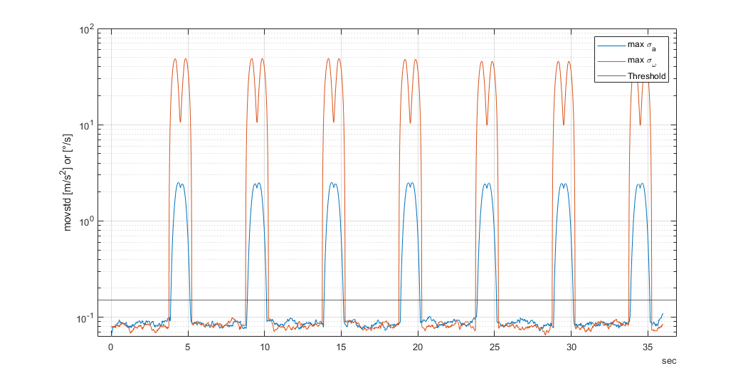
As mentioned earlier one method to detect zero velocity is to calculate the moving standard deviation with a window size of some \( N \) samples. If the standard deviation is below a certain threshold, we assume that the sensor is not moving.
The following plot shows the moving standard deviation for the simulated accelerometer and gyroscope measurements, where each value is the maximum of the standard deviation of the three axes. A window size of \( N = 100 \) samples was used and a threshold line at \( 0.15 \) is shown.
The implementation of the zero velocity detection with a window size of \( N = 100 \) samples and a threshold of \( 0.15 \) is given by
where acc and gyr are the accelerometer and gyroscope measurements, respectively.
The following plot shows the confusion matrix of the zero velocity detection.
Note that nearly ten percent of the samples are detected as not zero velocity although the true velocity is zero. This is due to the importance of having zero False Positives (lower left corner). The False Positives can be reduced by increasing the window length or decreasing the threshold. Obviously, if the window is long, the start and end of the zero velocity period will not be detected.
The EKF and RTS equations are identical to the ones derived in the previous section Part 4: Extended Kalman Filter. Please look them up there.
The Matlab implementation of this derivation is shown in derivation5Ekf6D.m.
pinv is used to calculate the pseudo-inverse of a matrix because the matrices are close to singular. Another method would be to use the Cholesky decomposition.USE_SENSITIVITY to true or false.VQF approach is the filter proposed in this paper which claims to be better than all considered literature methods, which include multiple Kalman approaches. In the results of the derivation5Ekf6D.m script, the VQF approach is not better than the EKF without sensitivity states.Since it's not possible to estimate the initial yaw angle without a magnetometer, the yaw of the first time step is set to the same value as the true yaw angle, i.e. the error at \( k=0 \) is only due to roll and pitch. The following plots show the results of the EKF and the RTS smoother with and without sensitivity states and also the VQF approach.
The following plot shows the total error of the orientation for the EKF and the RTS smoother with sensitivity states (with rng(1)). The error is calculated as the total angle between the true and estimated orientation without considering the direction of the rotation error (i.e. there is only one error for each time step).
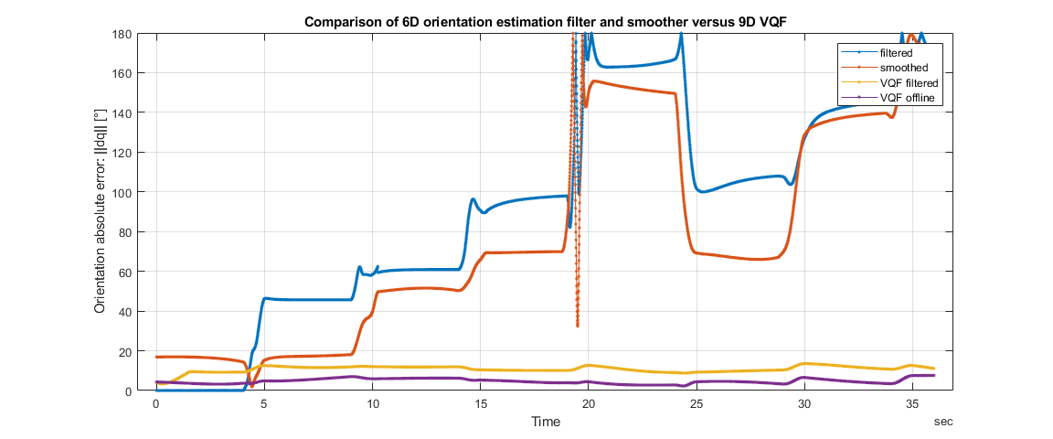
As we can see, the EKF and the RTS smoother with sensitivity states perform very bad. The error is very high and the orientation is not estimated correctly.
The following plot shows the total error of the orientation for the EKF and the RTS smoother without sensitivity states (with rng(1)). The error is calculated as the total angle between the true and estimated orientation without considering the direction of the rotation error (i.e. there is only one error for each time step).
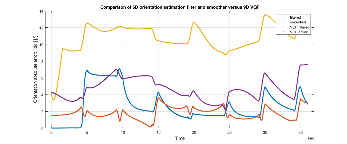
As we can see, the EKF and the RTS smoother without sensitivity states perform much better than with sensitivity states. The error is much lower and the estimated orientation is much closer to the true orientation. The RTS smoother performs better than the EKF (in the mean, as expected). The VQF approach is much worse than the EKF and the RTS smoother.
The following table shows the mean of the total error of the orientation for the EKF and the RTS smoother with and without sensitivity states. This data is based on 11 different random seeds (rng(x) with \( x = [0;10]\)), i.e. eleven different simulated sensor errors.
| Method | mean absolute error [°] |
|---|---|
| EKF with sensitivity states | 61.56 |
| RTS smoother with sensitivity states | 63.08 |
| EKF without sensitivity states | 4.56 |
| RTS smoother without sensitivity states | 2.64 |
| VQF Filter | 10.56 |
| VQF Smoother | 5.29 |
Obviously, the EKF and the RTS smoother without sensitivity states perform much better than with sensitivity states. The VQF approach is less accurate than the EKF and the RTS smoother without sensitivity states. The smoothing results could be further improved by introducing a orientation pseudo-measurement at one or more timesteps \( k \gg 1 \).
The EKF and the RTS smoother without sensitivity states perform much better than with sensitivity states. The VQF approach is less accurate than the EKF and the RTS smoother without sensitivity states. The smoothing results could be further improved by introducing a orientation pseudo-measurement at one or more timesteps \( k \gg 1 \). Based on the results, in the following section we will use the EKF filter and the RTS smoother without sensitivity states. Also, we finally add 3d position estimation to the filter.