Nichtlineare Ausgleichsrechnung¶

[1]:

import numpy as np
import matplotlib.pyplot as plt
from scipy.linalg import solve_triangular, qr
import sympy as sp

Modell¶

Daten

[2]:

data = np.array([
    [0.1, 0.3, 0.7, 1.2, 1.6, 2.2, 2.7, 3.1, 3.5, 3.9],
    [0.558, 0.569, 0.176, -0.207, -0.133, 0.132, 0.055, -0.090, -0.069, 0.027]
]).T

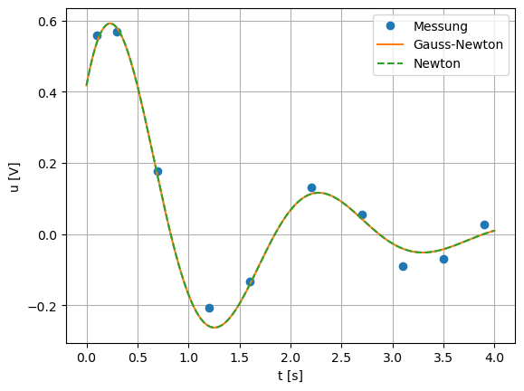
Das Modell ist gegeben durch eine gedämpfte Schwingung

\begin{equation}y(t;x_1,x_2,x_3,x_4) = x_1\,e^{-x_2 t}\sin(x_3 t+x_4).\end{equation}

Für die Daten sollen Amplitude, Dämpfung, Frequenz und Phase bestimmt werden.

[3]:

# Modellfunktion (direkt Numpy)
def y(t,x):
    a, tau, omega, phi = x
    return a*np.exp(-tau*t)*np.sin(omega*t+phi)

# Implementierung des Gradienten (direkt Numpy)
def dy(t,x):
    a, tau, omega, phi = x
    return np.array([np.exp(-tau*t)*np.sin(omega*t+phi),
                     -t*a*np.exp(-tau*t)*np.sin(omega*t+phi),
                     t*a*np.exp(-tau*t)*np.cos(omega*t+phi),
                     a*np.exp(-tau*t)*np.cos(omega*t+phi)]).T

# Implementierung der Hess'schen Matrix (direkt Numpy)
def Hy(t,x):
    a, tau, omega, phi = x
    return np.array([[[0,-ti*np.exp(-tau*ti)*np.sin(omega*ti+phi),ti*np.exp(-tau*ti)*np.cos(omega*ti+phi),np.exp(-tau*ti)*np.cos(omega*ti+phi)],
                     [-ti*np.exp(-tau*ti)*np.sin(omega*ti+phi),ti**2*a*np.exp(-tau*ti)*np.sin(omega*ti+phi),-ti**2*a*np.exp(-tau*ti)*np.cos(omega*ti+phi),-ti*a*np.exp(-tau*ti)*np.cos(omega*ti+phi)],
                     [ti*np.exp(-tau*ti)*np.cos(omega*ti+phi),-ti**2*a*np.exp(-tau*ti)*np.cos(omega*ti+phi),-ti**2*a*np.exp(-tau*ti)*np.sin(omega*ti+phi),-ti*a*np.exp(-tau*ti)*np.sin(omega*ti+phi)],
                     [np.exp(-tau*ti)*np.cos(omega*ti+phi),-ti*a*np.exp(-tau*ti)*np.cos(omega*ti+phi),-ti*a*np.exp(-tau*ti)*np.sin(omega*ti+phi),-a*np.exp(-tau*ti)*np.sin(omega*ti+phi)]] for ti in t])

[4]:

# Fehlerquadratsumme
def phi(data, x):
    t,yi = data.T
    Fi = y(t,x)-yi
    return 0.5*Fi.dot(Fi)

# Gradient Fehlerquadratsumme
def dphi(data, x):
    t,yi = data.T
    Fi = y(t,x)-yi
    dFi = dy(t,x)
    return dFi.T@Fi

# Hess'sche Matrix Fehlerquadratsumme
def Hphi(data, x, reduced = True):
    t,yi = data.T
    Fi = y(t,x)-yi
    dFi = dy(t,x)
    Hyi = Hy(t,x)
    s1 = dFi.T@dFi
    s2 = 0 if reduced else np.sum([Fi[k]*Hyi[k] for k in range(yi.shape[0])],axis=0)
    return s1 + s2

Gauss-Newton und Newton Verfahren¶

[5]:

# selber im Praktikum implementieren
from NichtlineareAusgleichsrechnungLib import GaussNewton

Eine minimal Stelle der Fehlerquadratsumme erfüllt die die Gleichung \(\nabla\phi(x) = 0\). Wir berechnen mit Hilfe des Newton-Verfahren die Nullstelle. Dazu benötigen wir die oben definierte Hess’sche Matrix:

[6]:

def Newton(data, x0, phi, dphi, Hphi,
           maxIter=100, maxDamp=20, tol=1e-12):
    # Daten
    t, yi = data.T
    # Initialisierung des Parameter Vektors
    x = np.array(x0)
    # Liste fuer die Visualisierung der Konvergenz
    res = []
    for k in range(maxIter):
        if k<3:
            # (reduzierte) Hess'sche Matrix von phi
            A = Hphi(data,x,reduced=True)
        else:
            # Hess'sche Matrix von phi
            A = Hphi(data,x,reduced=False)
        # Gradient von phi
        b = dphi(data,x)
        # Newton-Schritt
        q,r = qr(A,mode='economic')
        s = solve_triangular(r,q.T@b)
        # Daempfung, phi muss kleiner werden
        alpha = 1.
        for j in range(maxDamp):
            xn = x-alpha*s
            if phi(data,xn) < phi(data,x):
                break
            else:
                alpha /= 2
        x -= alpha*s
        res.append(np.linalg.norm(dphi(data,x)))
        print(k, phi(data,x), res[-1], alpha)
        if np.linalg.norm(s) < tol:
            break
    return x,res

[7]:

x0 = np.array([1, 1, 3, 1],dtype=float)
xN,resN = Newton(data,x0,phi,dphi,Hphi)

0 0.006673535239173661 0.07066924178449757 1.0
1 0.004033519639008082 0.007667311379775573 1.0
2 0.0039697638126295785 0.0013838504393927122 1.0
3 0.003963649748752298 1.6485434862469543e-05 1.0
4 0.003963649054560297 3.4785202919888354e-09 1.0
5 0.003963649054560273 1.5516887710921733e-16 1.0
6 0.003963649054560272 1.9299985848078835e-16 0.25

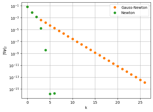
Im Vergleich dazu betrachten wir die Lösung bzw. das Konvergenz-Verhalten des Gauss-Newton Algorithmus gegeben aus der Vorlesung. Die eigene Implementierung des Gauss-Newton Algorithmus ist Inhalt des Praktikum.

[8]:

xGN,resGN = GaussNewton(data,x0,y,dy)

0 0.006673535239173671 0.07066924178449756
1 0.0040335196390080845 0.007667311379775534
2 0.003969763812629577 0.001383850439392612
3 0.003964376876659761 0.00043189264339680336
4 0.003963737754840471 0.00015315297340659568
5 0.003963659789483246 5.271531799257331e-05
6 0.003963650357168144 1.8446065026028378e-05
7 0.003963649212505831 6.408222596850327e-06
8 0.003963649073718184 2.2344040945342482e-06
9 0.003963649056883814 7.776815847694655e-07
10 0.003963649054842095 2.709242325054453e-07
11 0.003963649054594453 9.433741891124994e-08
12 0.0039636490545644125 3.2857208580372187e-08
13 0.003963649054560771 1.14424494661288e-08
14 0.00396364905456033 3.985091873460136e-09
15 0.0039636490545602795 1.3878456870227513e-09
16 0.003963649054560275 4.833400946087831e-10
17 0.003963649054560274 1.6832934015642728e-10
18 0.003963649054560274 5.86231170496666e-11
19 0.003963649054560272 2.0416286679951663e-11
20 0.003963649054560267 7.110299683392491e-12
21 0.0039636490545602735 2.4762243131069084e-12
22 0.003963649054560271 8.623606181540378e-13
23 0.003963649054560269 3.003270460861941e-13
24 0.003963649054560271 1.0453868873678433e-13
25 0.003963649054560267 3.646791165722058e-14
26 0.003963649054560276 1.2696633946590443e-14

[9]:

tp = np.linspace(0,4,400)
plt.plot(*data.T,'o',label='Messung')
plt.plot(tp,y(tp,xGN), label='Gauss-Newton')
plt.plot(tp,y(tp,xN),'--', label='Newton')
plt.legend()
plt.grid()
plt.xlabel('t [s]')
plt.ylabel('u [V]')
#plt.savefig('NonlinRegressBeispielSolution.pdf')
plt.show()

../_images/Gleichungen_NichtlineareAusgleichsrechnungBeispielSkript_15_0.png

[10]:

plt.semilogy(resGN, 'o', c='tab:orange', label='Gauss-Newton')
plt.semilogy(resN,'o', c='tab:green', label='Newton')
plt.legend()
plt.grid()
plt.xlabel('k')
plt.ylabel(r'$\|\nabla \varphi\|_2$')
#plt.savefig('NonlinRegressBeispielKonvergenz.pdf')
plt.show()

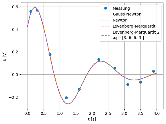
../_images/Gleichungen_NichtlineareAusgleichsrechnungBeispielSkript_16_0.png

Levenberg Marquardt¶

[11]:

from NichtlineareAusgleichsrechnungLib import LevenbergMarquardt

Das Levenberg-Marquardt Verfahren benutzt zwei Ansätze kombiniert. Zum einen wird eine Regularisierung eingeführt und zum andern eine Trust Region Strategie benutzt (vgl. Skript).

[12]:

xLM,resLM = LevenbergMarquardt(data,x0,y,dy)

0 USED 0.9806930724984753 0.02522309181409673 0.17285585253073918 0.5
1 USED 0.966743198838584 0.008653026324286795 0.038992518483582254 0.25
2 USED 1.0690298186175362 0.004742831395895376 0.014525297100761905 0.125
3 USED 0.9689610507864899 0.003998477441547046 0.004238121160033926 0.0625
4 USED 1.0587686404655003 0.003965149563202187 0.0006920225278408606 0.03125
5 USED 0.9703069931253844 0.003963737808783977 0.00015005328879465278 0.015625
6 USED 0.8231176366477855 0.003963656349909945 4.610316702023821e-05 0.0078125
7 USED 0.7175674870316264 0.003963649816848028 1.3789973649376374e-05 0.0078125
8 USED 0.6731120403436198 0.003963649142260981 4.85950466939716e-06 0.0078125
9 USED 0.6586292353941906 0.0039636490649735175 1.6356205271364175e-06 0.0078125
10 USED 0.6542237205365327 0.003963649055808716 5.732618016672834e-07 0.0078125
11 USED 0.6529533939512067 0.003963649054710364 1.9743631222088448e-07 0.0078125
12 USED 0.6529533939512067 0.0039636490545783346 6.873235821832852e-08 0.0078125
13 USED 0.6529533939512067 0.003963649054562442 2.3798520377686786e-08 0.0078125
14 USED 0.6529533939512067 0.003963649054560531 8.265112635232012e-09 0.0078125
15 USED 0.6529533939512067 0.003963649054560305 2.8658677079128567e-09 0.0078125
16 USED 0.6529533939512067 0.00396364905456028 9.94580074439072e-10 0.0078125
17 USED 0.6529533939512067 0.00396364905456028 3.4500234920859906e-10 0.0078125
18 USED 0.6529533939512067 0.003963649054560273 1.1970526892445235e-10 0.0078125
19 USED 0.6529533939512067 0.003963649054560278 4.1528487727630133e-11 0.0078125
20 USED 0.6529533939512067 0.00396364905456027 1.4408169131880016e-11 0.0078125
21 USED 0.6529533939512067 0.00396364905456027 4.99864980207953e-12 0.0078125
22 USED 0.6529533939512067 0.003963649054560273 1.7343600054359126e-12 0.0078125
23 USED 0.6529533939512067 0.003963649054560268 6.016996629540863e-13 0.0078125
24 USED 0.6529533939512067 0.003963649054560273 2.087165844251478e-13 0.0078125
25 USED 0.6529533939512067 0.003963649054560274 7.247123662743386e-14 0.0078125
26 USED 0.6529533939512067 0.003963649054560273 2.5215433981181632e-14 0.0078125

[13]:

x1 = np.array([3, 6, 6, 3],dtype=float)
xLM2,resLM2 = LevenbergMarquardt(data,x1,y,dy)

0 USED 1.0688949493208173 0.6046111148862408 0.8273909422867344 0.5
1 USED 0.9737610307872686 0.3747211303868591 0.2720130063224477 0.25
2 USED 0.7128631919430277 0.2563666206008889 0.13957511146131057 0.25
3 USED 0.4900585971435755 0.21770136422014721 0.1310297280092487 0.25
4 USED 1.0275298771905637 0.16497114046775874 0.08110172361955954 0.125
5 NOT  -4.249547548328965 0.16497114046775874 0.08110172361955954 0.25
6 USED 0.8725764875044045 0.13251205948189726 0.0991085112949658 0.125
7 USED 0.5247141798763945 0.10394987595977338 0.38433845837900554 0.125
8 USED 0.9987748295204908 0.06328659906475677 0.06187034873177772 0.0625
9 USED 0.9914348337268244 0.05541433147594083 0.037718410811648326 0.03125
10 USED 0.5397020835316607 0.05116622558523228 0.04707102905735394 0.03125
11 USED 0.4610701111309999 0.04963346243695535 0.047078692938088015 0.03125
12 USED 0.9190916385727865 0.046591895012284404 0.07354592948771659 0.015625
13 NOT  -17931912.43198623 0.046591895012284404 0.07354592948771659 0.03125
14 NOT  -19.225773477478008 0.046591895012284404 0.07354592948771659 0.0625
15 USED 0.9637337383230519 0.042054140670382587 0.04925316098536491 0.03125
16 NOT  -33.4960412829057 0.042054140670382587 0.04925316098536491 0.0625
17 USED 1.0953276240225318 0.03173672744281399 0.10852194461743497 0.03125
18 NOT  -2.3476148608466043 0.03173672744281399 0.10852194461743497 0.0625
19 USED 1.074103023624682 0.009493695403746826 0.08435009589846587 0.03125
20 USED 1.025107006335871 0.0040399450756643685 0.0063101402632417 0.015625
21 USED 1.1378258688272207 0.003966143774584509 0.0008295945011056233 0.0078125
22 USED 1.1509611095861016 0.003963746103141874 0.00017240958121187834 0.00390625
23 USED 1.091027250648086 0.003963653387765475 3.3364816706188546e-05 0.001953125
24 USED 0.9583117324706479 0.003963649321179371 8.947727420950248e-06 0.0009765625
25 USED 0.8008753067535109 0.003963649077879644 2.3916115374365196e-06 0.00048828125
26 USED 0.7051248082224726 0.003963649057075132 8.304052156718853e-07 0.00048828125
27 USED 0.6682218123536994 0.003963649054854386 2.733943968087441e-07 0.00048828125
28 USED 0.6682218123536994 0.003963649054595565 9.656213816456573e-08 0.00048828125
29 USED 0.6682218123536994 0.003963649054564545 3.3211205022775275e-08 0.00048828125
30 USED 0.6682218123536994 0.003963649054560796 1.1627612924616985e-08 0.00048828125
31 USED 0.6682218123536994 0.003963649054560335 4.036298846763535e-09 0.00048828125
32 USED 0.6682218123536994 0.003963649054560285 1.407959787605587e-09 0.00048828125
33 USED 0.6682218123536994 0.003963649054560274 4.898920785566606e-10 0.00048828125
34 USED 0.6682218123536994 0.0039636490545602735 1.7069005270244187e-10 0.00048828125
35 USED 0.6682218123536994 0.00396364905456027 5.942906732664566e-11 0.00048828125
36 USED 0.6682218123536994 0.00396364905456027 2.0699549134231818e-11 0.00048828125
37 USED 0.6682218123536994 0.0039636490545602735 7.208306366916543e-12 0.00048828125
38 USED 0.6682218123536994 0.00396364905456027 2.510455970506066e-12 0.00048828125
39 USED 0.6682218123536994 0.003963649054560274 8.742783832251762e-13 0.00048828125
40 USED 0.6682218123536994 0.003963649054560274 3.04508802929177e-13 0.00048828125
41 USED 0.6682218123536994 0.003963649054560266 1.0610663207321321e-13 0.00048828125
42 USED 0.6682218123536994 0.003963649054560274 3.6865907915161137e-14 0.00048828125
43 USED 0.6682218123536994 0.003963649054560277 1.2857108564914876e-14 0.00048828125

[14]:

tp = np.linspace(0,4,400)
plt.plot(*data.T,'o',label='Messung')
plt.plot(tp,y(tp,xGN), label='Gauss-Newton')
plt.plot(tp,y(tp,xN),'--', label='Newton')
plt.plot(tp,y(tp,xLM),'--', label='Levenberg-Marquardt')
plt.plot(tp,y(tp,xLM2),'--', label='Levenberg-Marquardt 2\n$x_0=$'+str(x1))
plt.legend()
plt.grid()
plt.xlabel('t [s]')
plt.ylabel('u [V]')
#plt.savefig('NonlinRegressBeispielSolution2.pdf')
plt.show()

../_images/Gleichungen_NichtlineareAusgleichsrechnungBeispielSkript_22_0.png

[15]:

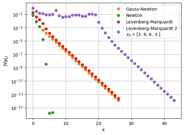
plt.semilogy(resGN, 'o', c='tab:orange', label='Gauss-Newton')
plt.semilogy(resN,'o', c='tab:green', label='Newton')
plt.semilogy(resLM,'o', c='tab:red', label='Levenberg-Marquardt')
plt.semilogy(resLM2,'o', c='tab:purple', label='Levenberg-Marquardt 2\n$x_0=$'+str(x1))
plt.legend()
plt.grid()
plt.xlabel('k')
plt.ylabel(r'$\|\nabla \varphi\|_2$')
#plt.savefig('NonlinRegressBeispielKonvergenz2.pdf')
plt.show()

../_images/Gleichungen_NichtlineareAusgleichsrechnungBeispielSkript_23_0.png

Aus dem Gauss-Newton Verfahren erhalten wir die Lösung:

[16]:

xGN

[16]:

array([0.73535605, 0.79620177, 3.07449929, 0.60418125])

\begin{equation}y(t;x_1,x_2,x_3,x_4) \approx 0.735\,e^{-0.8 t}\sin(3 t + 0.6).\end{equation}