3. Swiss-AL Tools#
3.1. Explore Corpus#
By using the tools in the Explore Corpus section, you can explore the content by letting the data guide you through the process. These modules are a good starting point when you have no specific assumptions about the data and want to let patterns emerge directly from your corpus.
3.1.1. Overview#
A click on Overview displays the corpus metadata and statistics, including:
corpus name
language
corpus type
time period
number of documents
number of tokens
number of documents per year
list of corpus sources (interactive pie chart)
list of corpus sources (interactive, searchable, and sortable table)
See examples for all corpora and their contents in Corpora.
3.1.2. Topics#
What are Topics?
Topics are clusters of words that frequently appear together in a set of documents and represent a common theme or subject.
In a collection of texts about different subjects, a topic model analyzes the words in these articles and tries to find groups of words that commonly appear together. Each word group (or topic) might correspond to a theme like storm, flood or climate_change without anyone manually labeling them.
We use Latent Dirichlet Allocation (LDA) to detect topics in a selected corpus Blei at al. 2003. LDA is a generative probabilistic model that represents documents as mixtures of topics, where each topic is a distribution over words. It is widely used for topic modeling due to its ability to handle large corpora efficiently and produce interpretable results.
Topics in Swiss-AL Platform
The Swiss-AL Platform provides pre-calculated topics for each corpus created with the Python package tomotopy. Additionally, when a user creats a subcorpus, automatically a model with 50 number of topics will be calculated.
All topic models are calculated using up to four consecutive words (lemmas) as the basic unit of analysis. We use TermWeight.IDF for weighting terms to be considered as topic keywords. This weighting method assigns lower importance to terms that appear in many documents across the corpus, as such terms are less useful for distinguishing between topics. Conversely, terms that occur in fewer documents receive a higher weight, making them more likely to characterize a specific topic.
Term weighting is based on Wilson et al. (2010). For topics visualisations in 2D and 3D format, we use tsne.
Topic Modeling View
Topic List: Contains topic numbers (Topic Nr.), a list of 25 keywords per topic (Words). Size(%) shows how prominent a topic is across the entire corpus. It is calculated by summing the topic probabilities across all documents and weighting them by document length.
Topic Network: Visualizes the topics in a 2D space. Similar topics are placed closed to each other. The bubble size depends on the number of documents associated with the topic. By hovering on individual bubbles, 5 most prominint keywords per topic are shown. A click on a bubble highlights the corresponding topic row in the Topic List.
💡 Note that:
Topic numbers (e.g., 1, 2, 3) are arbitrary and do not inherently carry any meaning.
It is common for one or two topics to act as background topics capturing words that do not strongly belong to any specific theme, often consisting of high-frequency, general-purpose terms.
If you want to know more about a particular topic, click on the topic number to see One-Topic View.
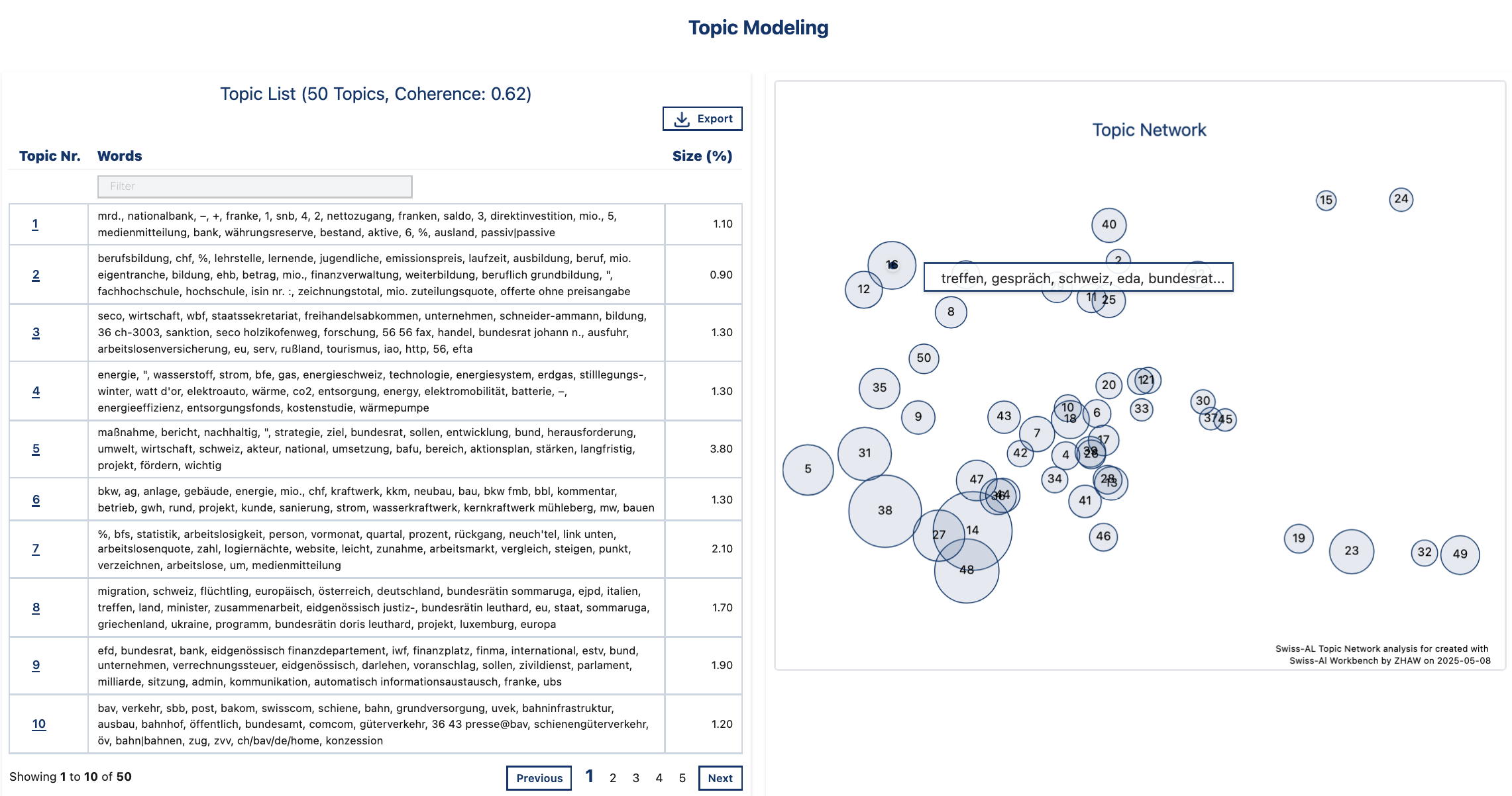 *Overview of topics in the corpus DE Demo Corpus *
One-Topic View
Top Words: Shows a list of keywords for the selected topic.
Topic Over Time: This feature visualizes the frequency of the selected topic over time by showing the proportion of all tokens in each time period that belong to the topic. Users can switch between monthly and yearly view.
Top 20 Documents: Displays the texts most strongly associated with this topic, based on the coherence score, which measures the semantic similarity among a topic’s top words.
Top 5 Similar Topics: Shows a list of the five most similar topics, calculated based on topic-term distributions. The similarity measure used is cosine similarity.
Top Sources for This Topic: Highlights the 10 sources in which this topic appears most prominently, ranked by the proportion of document’s tokens that occur in the topic.
Topic Proportions by Category: Shows the proportion of tokens that are assigned to the topic divided by the total number of tokens in that category (e.g. media type, social system, etc.).
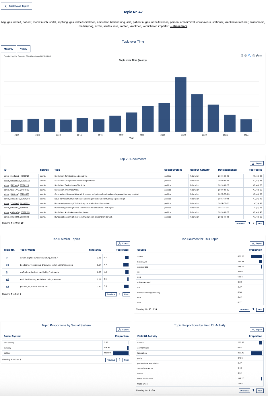 One-topic view: “bag, gesundheit, patient, medizinisch, spital,… “
3.1.3. Keywords#
What are keywords?
The tool Keywords identifies terms that occur considerably more frequently in one corpus (study corpus) compared to another corpus (reference corpus). In the Swiss-AL Platform, the keywords are determined using Log Likelihood Ratio (LLR).
Log Likelihood Ratio (LLR) measures how strongly a word is associated with one corpus compared to another corpus. In keyword analysis, it helps identify words that occur significantly more often in a target corpus than would normally be expected based on a reference corpus.
For example, if the word lockdown appears much more frequently in a corpus of COVID-19 news articles than in a general news corpus, the word will receive a high LLR score and can be considered a keyword of the COVID-19 corpus.
Unlike simple frequency counts, LLR takes corpus size into account and estimates whether the difference in frequency is likely to be meaningful rather than random.
In the Swiss-AL Platform, keywords are only available for subcorpora.
When a user creates a subcorpus, keywords are calculated relative to the parent corpus, which serves as the reference corpus, with the overlapping part between the selected subcorpus and the parent corpus excluded.
3.1.4. Semantic Space#
With this tool, users can search for semantically similar words by looking at nearest neighbors (words occurring in similar contexts). A semantic space is a mathematical representation of word meanings, where words (or phrases) are mapped to points in a multi-dimensional space based on their relationships with other words. In this space, words with similar meanings or usage tend to be closer together.
The nearest neighbors search produces:
Diagrams visualizing the vector space in both 2D and 3D (up to 5,000 most frequent words in the corpus);
A table displaying the cosine similarity values between the searched word(s) and their closest neighbors in the vector space.
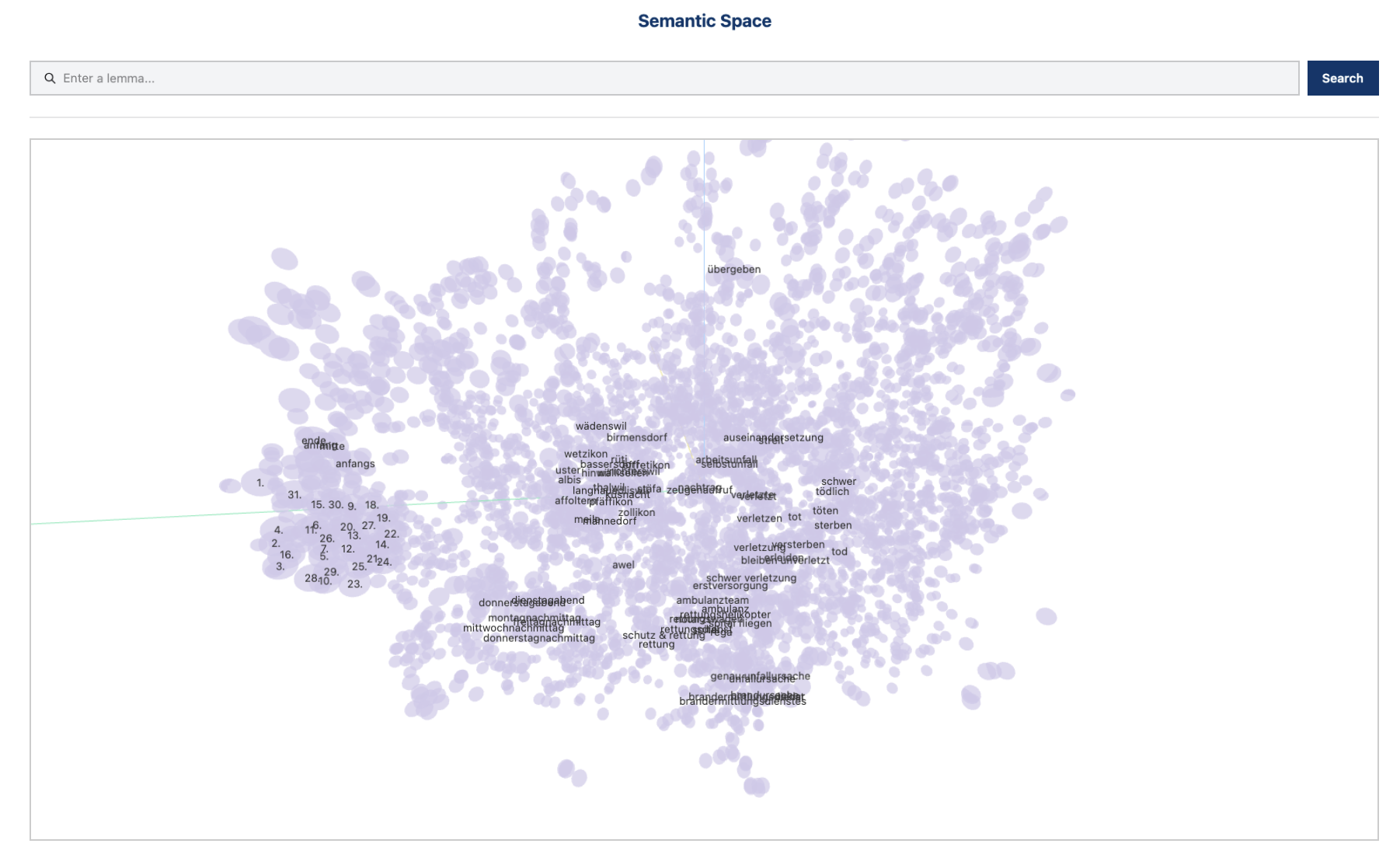 Semantic space in corpus “German Demo Corpus”
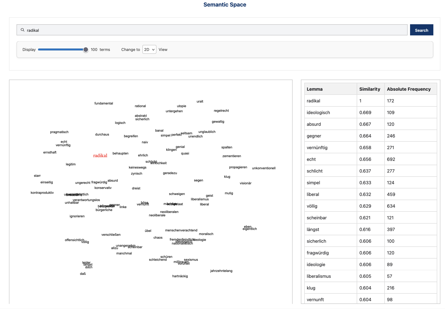 Semantic neighbors for “radikal” ‘radical’ in the corpus “German Demo Corpus”
To ensure reliable semantic representations, word embedding models are generated for subcorpora only when the corpus contains at least 10 million tokens.
You can learn more about the potential of word embeddings for discourse analysis in Bubenhofer et al. 2019. If you would like to read more on the general principal behind word embeddings, we recommend Lenci 2018.
3.2. Search Corpus#
By using the tools in the Search Corpus section, you can look for specific terms of interest and inspect their frequency distribution and documents in which they occur. The Swiss-AL Platform provides three different Search Modes: Quick Search, Basic Search and Advanced Search. Please take a moment to get to know these modes before you start searching. And don’t hesitate to explore the Advanced Search mode — it lets you use regular expressions (regex) to create more complex and powerful queries. You can also search for named entities, corpus annotations, and even longer or more specific formulations to refine your results.
3.2.1. Distribution of Words#
The tool Distribution of Words is divided in four modules:
Frequency Table: this functionality shows the most frequent forms for your search term. If you are interested in the frequency of the main form (lemma) of your search, select Group by lemma. The relative frequency is measured as Word per Million (WPM). WPM is a way to express the relative frequency of a word or term in a text or corpus, standardized per 1,000,000 words. This measure is commonly used in corpus linguistics since it allows word comparison across texts of different lengths. Here is a rough idea to help you put WPM values in perspective:
How frequent is frequent?
Very common function words
Words like the, and, of, in
50,000 – 100,000 WPM (5–10% of all words)
Example: the occurs about 60,000 times per 1,000,000 words
Common content words
Words like house, work, day
1,000 – 5,000 WPM
Less frequent or specialized words
Words like photosynthesis, quantum, serendipity
10 – 500 WPM
Rare words
Very uncommon words, technical terms, names
<10 WPM, sometimes only a single occurrence in a million words
Word Distribution over Time: this functionality shows the distribution of your search term through time. You can adjust the time span by interacting with the graph. A 7-day moving average takes the average number of occurrences of the searched term within 7 days. It smooths out daily fluctuations to show the overall trend more clearly.
Grouped by Source: this functionality shows the distribution of your search term throughout all sources in your corpus.
Grouped by Category: this functionality shows the distribution of your search term throughout categories in your corpus. For instance, for media texts: category 1 is publisher or media type. The latter is further divided in category 2: daily/online newspaper, weekly/magazine, special interest magazine and radio/tv.
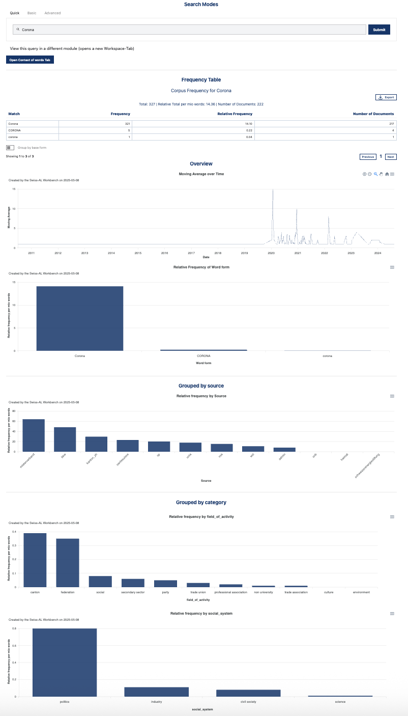 *Distribution of Words for the search term Corona *
💡 See examples for all categories in Section Corpora.
💡 The relative frequencies shown in the diagrams indicate the total number of hits found in a specific category divided by the total number of hits in the corpus.
3.2.2. Context of Words#
The tool Context of Words allows you to view text segments containing your search term. This tool has two modes:
KWIC View: Per default users can see 5 tokens left and right of your search term. You can add more context — up to two sentences on both sides. This view is traditionally used in corpus linguistics (where it is usually called KWIC for Key Word In Context) and it is useful if you are interested in the contexs in which your search term occures throughout the corpus. You can sort the table on ascending or descending the columns.
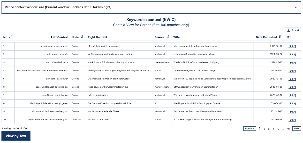 KWIC View for the search term “Corona”
3.2.3. Distribution in Documents#
Document View: This view has been developed for facilitating the search for relevant documents. In comparison to the KWIC View, which displays a row for each individual occurrence of the searched term in the corpus, the Document View shows one row for each document that contains the searched term(s). Additionaly, it shows:
Distribution (Distribution of your search term in document): Each document is divided into ten equally sized segments along the horizontal bar. The blue squares represent the approximate positions of the search term(s) in the text. The color intensity corresponds to the frequency of hits in the respective segment divided by the total frequency of hits in the document. You can sort this table to explore, for example, whether your search terms occur more frequently at the beginning or end of a given document.
Document Keywords: Words that occur in the document more frequently than in the corpus, adjusted for text length (using Log Ratio).
Text metadata, including titles, which will also likely help you find the relevant documents.
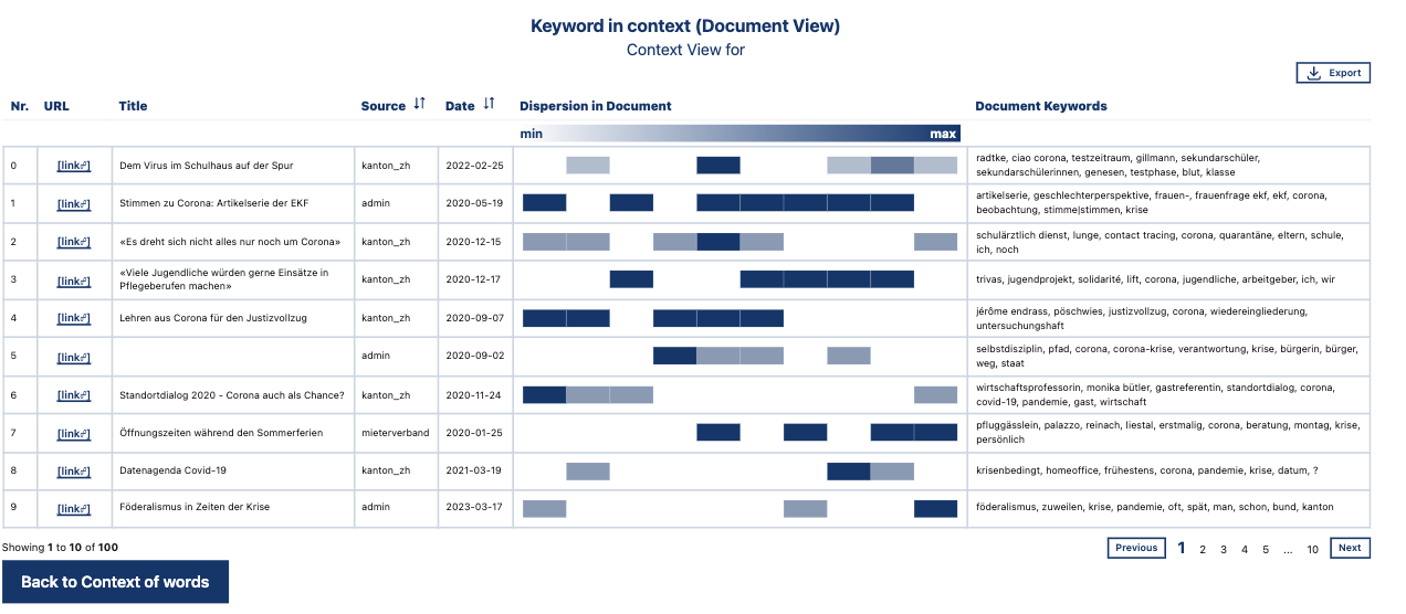 Document View for the search term “Corona”
💡 Note that:
Document keywords in Context of Words differ from corpus keywords created with Keywords.
3.2.4. Common Pairings#
Common pairings, also called collocations or co-occurrences, are words that frequently occur together in a language. Such recurring combinations can reveal conventional and meaningful patterns of language use.
To identify these pairings, we use the statistical association measure LogDice.
LogDice measures the strength of association between two terms based on how often they co-occur. We define co-occurring as appearing within the same context window, consisting of n-words before and after the search term.
By default, if you search for common pairings with the term Corona, the tool searches for all lemmas that occur within a window of five words before and five words after Corona. You can adjust the settings to allow context windows of up to ten tokens before and after the search term.
By default, the tool displays lemmas, but you can change the settings to search for word forms instead (i.e. inflected forms).
An important advantage of LogDice is that it is independent of corpus size. This means that LogDice scores can be compared across different corpora, even if the corpora differ greatly in size.
 Common Pairings for the search term “Migration”