Energie Erhaltung

import numpy as np
import matplotlib.pyplot as plt
from sympy import *

Modell Beispiel

Als Modellbeispiel betrachten wir das Anfangswertproblem

\[\begin{split}\begin{split} \dot{x}(t) & = y(t)\\ \dot{y}(t) & = -x(t) \end{split}\end{split}\]

mit \(x(0)=0, y(0)=1\). Die analytische Lösung ist gegeben durch

\[(x(t),y(t)) = (\sin(t),\cos(t)).\]

Die Lösung erfüllt

\[E = x(t)^2 + y(t)^2 \equiv 1\quad \forall t\in\mathbb{R}.\]

Ein numerisches Verfahren, welches die Energie \(E\) (vgl. Skript) erhält, nennen wir konservativ.

def f(t,x):
    return np.array([x[1],-x[0]])

t,x1,x2,y1,y2,h = symbols('t,x1,x2,y1,y2,h')

Implizit Euler

Wir betrachten die implizite Euler Methode:

\[\begin{split}\begin{pmatrix}x_{n+1}\\y_{n+1}\end{pmatrix} = \begin{pmatrix}x_{n}\\y_{n}\end{pmatrix} + h\cdot f\left(t+h,\begin{pmatrix}x_{n+1}\\y_{n+1}\end{pmatrix}\right)\end{split}\]

und berechnen algebraisch (das System ist linear!) die Lösung für den neuen Zeitschritt:

sol=solve(np.array([x2,y2]) - np.array([x1,y1]) - h*f(t+h,[x2,y2]),[x2,y2])
sol

{y2: (-h*x1 + y1)/(h**2 + 1), x2: (h*y1 + x1)/(h**2 + 1)}

Damit folgt für \(x_{k+1}^2+y_{k+1}^2\):

simplify((x2.subs(sol))**2+(y2.subs(sol))**2)

$\displaystyle \frac{x_{1}^{2} + y_{1}^{2}}{h^{2} + 1}$

In jedem Schritt „verbraucht“ das Verfahren Energie und ist somit nicht konservativ!

Implizite Mittelpunkt-Regel

Für die implizite Mittelpunkt-Regel gilt (in der Steigungsform):

\[\begin{split}\begin{split}\begin{pmatrix}r_{x}\\r_{y}\end{pmatrix} & = f\left(t+\frac{h}{2}, \begin{pmatrix}x_{n}\\y_{n}\end{pmatrix} + \frac{h}{2}\cdot \begin{pmatrix}r_{x}\\r_{y}\end{pmatrix}\right)\\ \begin{pmatrix}x_{n+1}\\y_{n+1}\end{pmatrix} & = \begin{pmatrix}x_{n}\\y_{n}\end{pmatrix} + h \cdot \begin{pmatrix}r_{x}\\r_{y}\end{pmatrix}\end{split}\end{split}\]

Die Lösung für den neuen Zeitschritt:

t,x1,x2,y1,y2,rx,ry,h = symbols('t,x1,x2,y1,y2,rx,ry,h')

sol=solve(np.array([rx,ry]) - f(t+h/2,np.array([x1,y1])+h/2*np.array([rx,ry])),[rx,ry])
sol

{ry: -(2*h*y1 + 4*x1)/(h**2 + 4), rx: (-2*h*x1 + 4*y1)/(h**2 + 4)}

x2 = x1+h*rx
y2 = y1+h*ry

Damit folgt für \(x_{k+1}^2+y_{k+1}^2\):

simplify((x2.subs(sol))**2+(y2.subs(sol))**2)

$\displaystyle x_{1}^{2} + y_{1}^{2}$

Die Energie bleibt damit erhalten. Das Verfahren ist konservativ.

Implizite Trapezmethode

Für die implizite Trapezmethode gilt (in der Steigungsform):

\[\begin{split}\begin{pmatrix}x_{n+1}\\y_{n+1}\end{pmatrix} = \begin{pmatrix}x_{n}\\y_{n}\end{pmatrix} + \frac{h}{2} \cdot \left(f\left(t, \begin{pmatrix}x_{n}\\y_{n}\end{pmatrix}\right)+f\left(t+h, \begin{pmatrix}x_{n+1}\\y_{n+1}\end{pmatrix}\right)\right)\end{split}\]

Die Lösung für den neuen Zeitschritt:

t,x1,x2,y1,y2,h = symbols('t,x1,x2,y1,y2,h')

sol=solve(np.array([x2,y2]) - np.array([x1,y1]) - h/2*(f(t,np.array([x1,y1]))+f(t+h,np.array([x2,y2]))),[x2,y2])
sol

{y2: (-h**2*y1 - 4*h*x1 + 4*y1)/(h**2 + 4),
 x2: (-h**2*x1 + 4*h*y1 + 4*x1)/(h**2 + 4)}

Damit folgt für \(x_{k+1}^2+y_{k+1}^2\):

simplify((x2.subs(sol))**2+(y2.subs(sol))**2)

$\displaystyle x_{1}^{2} + y_{1}^{2}$

Die Energie bleibt damit erhalten. Das Verfahren ist ebenfalls konservativ.

Verfahren nach Hammer-Hollingsworth

Genauso kann gezeigt werden, dass das zweistufige Verfahren nach Hammer-Hollingsworth ebenso konservativ ist:

from sympy.matrices import Matrix

def f(t,x):
    return Matrix([x[1],-x[0]])

t,x1,x2,y1,y2,r1x,r1y,r2x,r2y,h = symbols('t,x1,x2,y1,y2,r1x,r1y,r2x,r2y,h')

r1 = Matrix([r1x,r1y])
r2 = Matrix([r2x,r2y])

cHH = Matrix([(3-sqrt(3))/6,(3+sqrt(3))/6])
aHH = Matrix([[1/4,(1/4-sqrt(3)/6)],[(1/4+sqrt(3)/6),1/4]])
bHH = Matrix([1/2,1/2])

Da wir es hier mit einem zwei stufigen Verfahren zu tun haben, sind die die beiden Richtungsvektoren \(r_1, r_2\) gesucht. Wir erhalten daher im Beispiel ein Gleichungssystem mit 4 Unbekannten \((r_{1,x}, r_{1,y}), (r_{2,x}, r_{2,y})\):

sol=solve([r1-f(t+cHH[0]*h,Matrix([x1,y1])+h*(aHH[0,0]*r1+aHH[0,1]*r2)),
           r2-f(t+cHH[1]*h,Matrix([x1,y1])+h*(aHH[1,0]*r1+aHH[1,1]*r2))],[r1x,r1y,r2x,r2y])
sol

{r1x: (-3.46410161513775*h**3*x1 + 8.78460969082653*h**2*y1 - 30.4307806183469*h*x1 + 144.0*y1)/(h**4 + 12.0*h**2 + 144.0),
 r1y: (-3.46410161513775*h**3*y1 - 8.78460969082653*h**2*x1 - 30.4307806183469*h*y1 - 144.0*x1)/(h**4 + 12.0*h**2 + 144.0),
 r2x: 2.0*(1.73205080756888*h**3*x1 - 16.3923048454133*h**2*y1 - 56.7846096908265*h*x1 + 72.0*y1)/(h**4 + 12.0*h**2 + 144.0),
 r2y: 2.0*(1.73205080756888*h**3*y1 + 16.3923048454133*h**2*x1 - 56.7846096908265*h*y1 - 72.0*x1)/(h**4 + 12.0*h**2 + 144.0)}

x2 = x1 + h*bHH.dot([r1x,r2x])
y2 = y1 + h*bHH.dot([r1y,r2y])

Damit folgt für \(x_{k+1}^2+y_{k+1}^2\):

simplify((x2.subs(sol))**2+(y2.subs(sol))**2)

$\displaystyle 1.0 x_{1}^{2} + 1.0 y_{1}^{2}$

Die Energie bleibt damit erhalten. Das Verfahren ist ebenfalls konservativ.

Klassisches Runge-Kutta Verfahren 4. Ordnung

Zum Abschluss betrachten wir das klassische Runge-Kutta Verfahren 4. Ordnung.

def f(t,x):
    return np.array([x[1],-x[0]])

t,x1,x2,y1,y2,h = symbols('t,x1,x2,y1,y2,h')

r1 = f(t,np.array([x1,y1]))
r2 = f(t+h/2,np.array([x1,y1])+h/2*r1)
r3 = f(t+h/2,np.array([x1,y1])+h/2*r2)
r4 = f(t+h,np.array([x1,y1])+h*r3)

[x2,y2] = np.array([x1,y1]) + h/6*(r1+2*r2+2*r3+r4)

Damit folgt für \(x_{k+1}^2+y_{k+1}^2\):

E = factor((x2.subs(sol))**2+(y2.subs(sol))**2)
E

$\displaystyle \frac{\left(x_{1}^{2} + y_{1}^{2}\right) \left(h^{8} - 8 h^{6} + 576\right)}{576}$

kappa = lambdify(h,E.subs({x1:1,y1:0}))

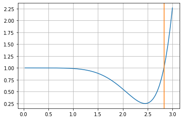
Nur mit einer Schrittweite von \(h=2\sqrt{2}\) oder \(h=0\) ist das Verfahren konservativ! Für kleine Schrittweiten ist das Verfahren jedoch nahezu konservativ. Der Fehler geht sehr schnell mit \(h^6\) gegen Null.

solve(E.subs({x1:1,y1:0})-1,h)

[0, -2*sqrt(2), 2*sqrt(2)]

hs = 10**np.linspace(-1.5,np.log10(3),300)
plt.plot(hs,kappa(hs))
plt.axvline(2*np.sqrt(2),c='tab:orange')
plt.grid()