Beispiel Anwendung der stetigen Abhängigkeit von Parameter

Gesucht ist der Parameter \(\alpha\) so, dass \(y(1) = 1\) gilt, wobei \(y(x)\) Lösung des Anfangswertproblem

\[\begin{split}\begin{split}y'(x) & = \cos(\alpha\, y(x)^2)\\ y(0) & = 0\end{split}\end{split}\]

ist. Da die Lösung der Differentialgleichung nicht analytisch berechnet werden kann, soll die Lösung numerisch berechnet werden. Dazu wird die Funktion \(G(\alpha)\) wie folgt definiert:

\[G(\alpha) = y(1,\alpha) - 1.\]

Gesucht ist somit \(\alpha\) so, dass \(G(\alpha) = 0\) erfüllt ist. Mit dem Newton Verfahren folgt

\[\alpha_{n+1} = \alpha_n - \frac{G(\alpha_n)}{G'(\alpha_n)}.\]

Für \(G'(\alpha)\) folgt

\[G'(\alpha) = \partial_\alpha y(1,\alpha).\]

Es wird daher die Partielle Ableitung der Lösung nach dem Paramter \(\alpha\) benötigt. Da \(y(x,\alpha)\) nur numerisch verfügbar ist, muss die Ableitung numerisch berechnet werden. Durch Ableiten der Differentialgleichung nach \(\alpha\) erhält man die Differentialgleichung für die partielle Ableitung:

\[\begin{split}\begin{split}\partial_\alpha y'(x,\alpha) & = -\sin(\alpha\, y(x,\alpha)^2)\cdot (y(x,\alpha)^2 + 2\,\alpha\, y(x,\alpha)\, \partial_\alpha y(x,\alpha))\\ \partial_\alpha y(0,\alpha) & = 0\end{split}\end{split}\]

In jedem Newton-Schritt muss daher das Anfangswertproblem

\[\begin{split}\begin{split} y'(x,\alpha) & = \cos(\alpha\, y(x,\alpha)^2)\\ \partial_\alpha y'(x,\alpha) & = -\sin(\alpha\, y(x,\alpha)^2)\cdot (y(x,\alpha)^2 + 2\,\alpha\, y(x,\alpha)\, \partial_\alpha y(x,\alpha))\\ y(0,\alpha) & = 0\\ \partial_\alpha y(0,\alpha) & = 0\end{split}\end{split}\]

gelöst werden, es gilt \(y'(x,\alpha) = \partial_x y(x,\alpha)\).

import numpy as np
import matplotlib.pyplot as plt

from hammerholingsworth import classicRungeKutta

In der numerischen Umsetzung ist \(y\) vektorwertig, gegeben durch \((y(x,\alpha), \partial_\alpha y(x,\alpha))\). Daher der Lösung der Differentialgleichung und der partiellen Ableitung nach \(\alpha\) der Lösung.

def f(x, y, alpha):
    return np.array([
        np.cos(alpha*y[0]**2),
        -np.sin(alpha*y[0]**2)*y[0]*(y[0]+2*alpha*y[1])
    ])

Initialisierung

h=1e-3
alpha = 1
y0 = np.array([0,0])
xk,yk = classicRungeKutta(2, h, y0, lambda x,y: f(x,y,alpha))

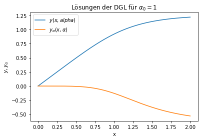
plt.plot(xk,yk[:,0],label=r'$y(x,alpha)$')
plt.plot(xk,yk[:,1],label=r"$y_\alpha(x,\alpha)$")
plt.legend()
plt.xlabel('x')
plt.ylabel(r'$y, y_\alpha$')
plt.title(r'Lösungen der DGL für $\alpha_0 = 1$')
plt.show()

Newton Verfahren für \(y(1,\alpha) = 1\):

\[\alpha_{n+1} = \alpha_n - \frac{G(\alpha_n)}{G'(\alpha_n)}\]

tol = 1e-13
nmax = 10
n = 0
G = yk[-1,0]-1
while np.abs(G) > tol and n < nmax:
    xk,yk = classicRungeKutta(2, h,y0,lambda x,y: f(x,y,alpha))
    G = yk[-1,0]-1 # G(alpha) = y(1)-1
    dG = yk[-1,1]  # G'(alpha) = dy/dalpha(1)
    alpha -= G/dG
    n += 1
    print(alpha, G)

1.416619566195272 0.22075705518863642
1.539251182137493 0.04238656475250324
1.5465865355959174 0.0022711596877358353
1.546610046426537 7.233093613390196e-06
1.5466100466664754 7.381539823825278e-11
1.5466100466664798 1.3322676295501878e-15

plt.plot(xk,yk[:,0],label=r'$y(x,alpha)$')
plt.legend()
plt.xlabel('x')
plt.ylabel(r'$y, y_\alpha$')
plt.title(r'Lösungen der DGL für $y(1,\alpha) = 1$')
plt.show()

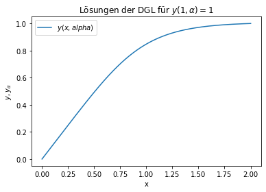
Mit \(\alpha = 0.03161911700972918\) wird die Bedingung \(y(1) = 1\) erfüllt.