
Explore Corpus#
Use these tools when you have no specific assumptions about the data and want patterns to emerge directly from your corpus.
Corpus metadata and statistics at a glance.
Clusters of words that recur together and point to a common theme.
Terms that are unusually frequent in one corpus compared to another.
Words that occur in similar contexts, and how close they sit to each other.
Overview#
Overview is the first place to look when you open a corpus you do not know, and the place to return to after creating a subcorpus. What a corpus contains shapes what its results mean: a frequency trend reads differently in a collection that ends in 2020 than in one that runs to last month, and a finding about “public discourse” reads differently if most documents come from a handful of sources. Checking the number of tokens also tells you whether a subcorpus is large enough for the tools that have size requirements.
A click on Overview displays the corpus metadata and statistics:
corpus name
language
corpus type
time period
number of documents
number of tokens
number of documents per year
list of corpus sources, as an interactive pie chart
list of corpus sources, as an interactive, searchable, sortable table
date of corpus creation
parent corpus (only for subcorpora)
Important
Corpus type is more than a descriptive label. It determines how the corpus sources are subcategorized, and therefore which categories are available when you group results in Distribution of Words. Before working with a corpus, read what its type means in Corpora.
Topics#
Topics are clusters of words that frequently appear together in a set of documents and represent a common theme or subject. In a collection of texts about different subjects, a topic model algorithm analyses the words in these articles and finds groups of words that commonly appear together. Each group might correspond to a theme such as storm, flood, or climate_change — without anyone labelling it manually. For the corpora in Swiss-AL, we use LDA, the most common topic modeling algorithm.
How topics are calculated in Swiss-AL
Topics are detected using Latent Dirichlet Allocation (LDA), a generative probabilistic model that represents documents as mixtures of topics, where each topic is a distribution over words. LDA is widely used because it handles large corpora efficiently and produces interpretable results (Blei et al. 2003).
The platform provides pre-calculated topics for each corpus, created with the Python package tomotopy. When you create a subcorpus, a model with 50 topics is calculated automatically.
All topic models use up to four consecutive words (lemmas) as the basic unit of analysis. Terms are weighted with TermWeight.IDF, which assigns lower importance to terms appearing in many documents across the corpus, since these are less useful for distinguishing between topics. Terms occurring in fewer documents receive a higher weight, making them more likely to characterise a specific topic. Term weighting follows Wilson et al. 2010.
Topic visualisations in 2D and 3D use t-SNE.
How LDA detects topics
Suppose we have a collection of climate texts we are unfamiliar with, and we want to know which themes they address without reading all of them.
Step 1 — Random topic assignment
LDA begins by assigning every word in every document to a random topic. At this point nothing is meaningful yet.
Document |
Text |
Initial assignment |
|---|---|---|
D1 |
The glacier is melting quickly |
glacier → T1, melting → T2, quickly → T3 |
D2 |
Rising temperatures and stronger storms |
rising → T2, storms → T1 |
Step 2 — Iterative refinement
The model then runs many iterations, reassigning each word to a topic based on the topics of the words around it. This procedure is called Gibbs sampling.
Document |
After several iterations |
|---|---|
D1 |
glacier → T1, melting → T1, quickly → T1 |
D2 |
rising → T2, storms → T2 |
Words that frequently appear together now share a topic: T1 has collected glacier, melting, quickly, and T2 has collected rising, storms.
Step 3 — Probability adjustment
Two probabilities drive each reassignment:
How often does this word appear in this topic? If glacier occurs mostly in T1, it will tend to stay there.
How often does this topic appear in this document? If a document consists mostly of T1 words, new words in it will tend to be assigned to T1.
Document |
Topic 1 |
Topic 2 |
|---|---|---|
D1 — The glacier is melting quickly |
80% |
20% |
D2 — Rising temperatures and stronger storms |
15% |
85% |
Step 4 — Convergence
After many iterations, words settle into stable topics. Every document is now a mixture of topics, and every topic has its characteristic words.
Topic 1 — glacier, melting, drought, sea-level, permafrost, erosion
Topic 2 — storm, hurricane, heatwave, flood, temperature, rainfall
The names climate effects and extreme weather are ours, not the model’s. LDA produces the word groups; interpreting and labelling them is the analyst’s work.
Using Topics#
When you open Topics, you see two panels side by side.
Topic List contains topic numbers (Topic Nr.) and 25 keywords per topic (Words). Size (%) shows how prominent a topic is across the entire corpus, calculated by summing topic probabilities across all documents and weighting them by document length.
Topic Network visualises the topics in 2D space. Similar topics sit close together, and bubble size reflects the number of documents associated with the topic. Hovering over a bubble shows the five most prominent keywords; clicking one highlights the corresponding row in the Topic List.
Tip
Topic numbers are arbitrary and carry no inherent meaning.
It is common for one or two topics to act as background topics, capturing high-frequency, general-purpose words that do not strongly belong to any theme.
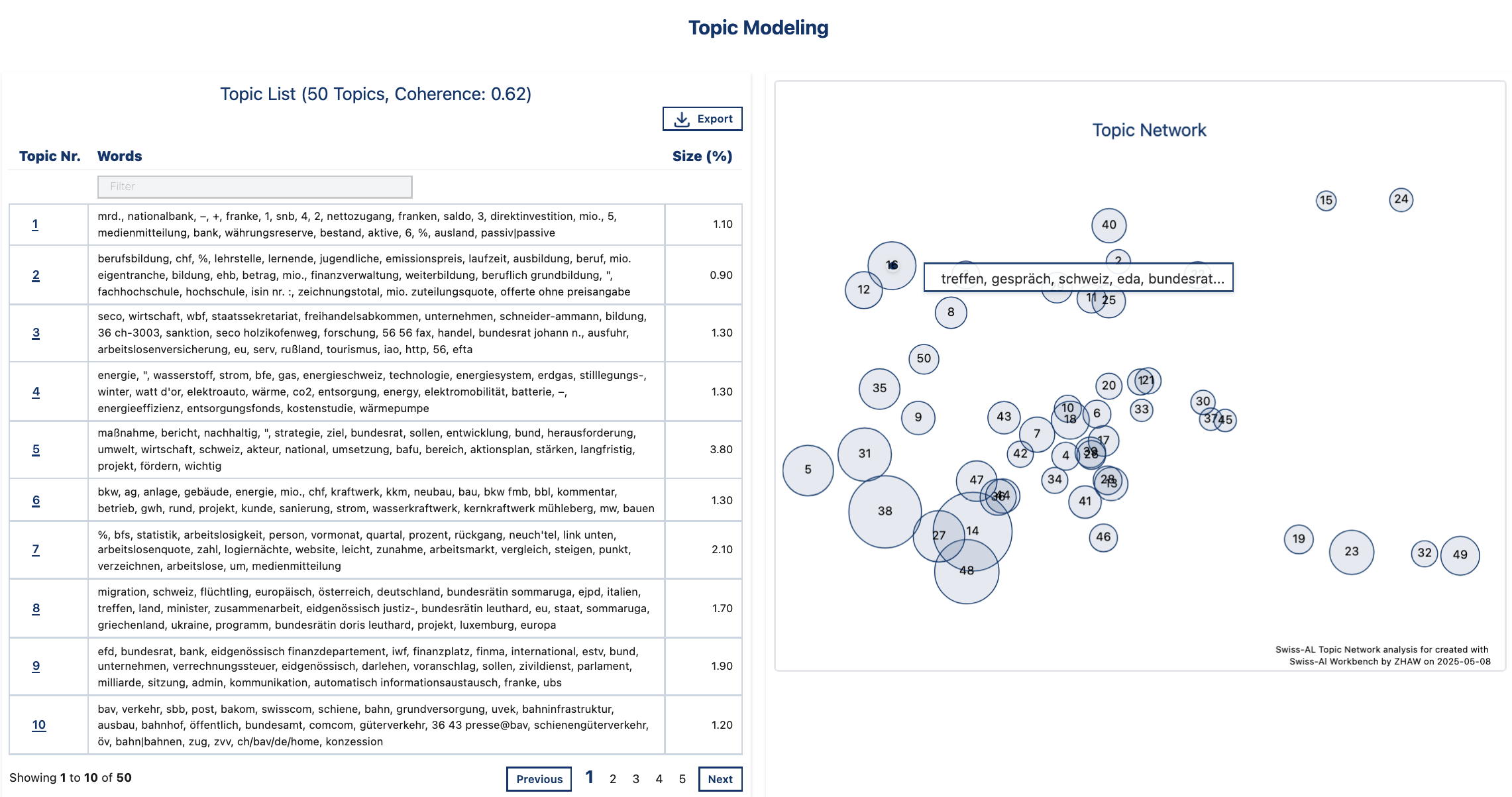
Fig. 8 Overview of topics in the DE Demo Corpus.#
To learn more about a particular topic, click its topic number to open the One-Topic View.
One-Topic View#
In this view, you can inspect individual topics in more detail.
Top Words — keywords for the selected topic (the same as in the Topic List).
Topic Over Time — the proportion of all tokens in each time period that belong to the topic. You can switch between monthly and yearly views.
Top 20 Documents — the texts most strongly associated with this topic, based on the coherence score, which measures semantic similarity among a topic’s top words.
Top 5 Similar Topics — the five most similar topics, calculated from topic-term distributions using cosine similarity.
Top Sources for This Topic — the ten sources in which the topic appears most prominently, ranked by the proportion of each document’s tokens that occur in the topic.
Topic Proportions by Category — the proportion of tokens assigned to the topic relative to all tokens in that category, such as media type or social system (categories depend on the corpus type, see Corpora).
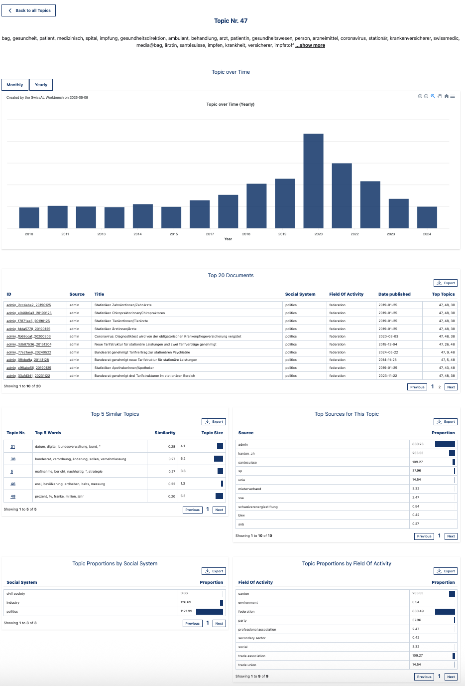
Fig. 9 One-topic view for the topic bag, gesundheit, patient, medizinisch, spital.#
Learn more
A short video introduction to topic modelling is available in Open Educational Resources.
Keywords#
The Keywords tool identifies terms that occur considerably more frequently in one corpus (the study corpus) than in another (the reference corpus).
For example, if the word lockdown appears much more often in a corpus of COVID-19 news articles than in a general news corpus, it will score highly and can be considered a keyword of the COVID-19 corpus.
Keywords are presented as a table (showing the keywords, their absolute frequency in the study corpus and ther Log Likelihood value) and a wordcloud. The size of a keyword in the wordclous is based on its Log Likelihood value.
Important
Keywords are available for subcorpora only. The corpora provided by the platform do not have a keyword analysis, so to use this tool you first need to create a subcorpus of your own.
Every subcorpus is derived from a larger corpus by filtering it, and that larger corpus is its parent corpus. In a keyword analysis your subcorpus acts as the study corpus and its parent acts as the reference corpus. The documents the two have in common are excluded from the reference side, so the comparison is between your selection and the rest of the parent corpus — not against a collection that already contains your selection.
How keywords are calculated
Keywords are determined using the Log Likelihood Ratio (LLR), also written G². It asks a simple question: if this word were equally at home in both corpora, how surprised should we be by the frequencies we actually observe? LLR measures how confident we can be that a frequency difference is not due to chance. It does not measure how large that difference is.
Step 1 — What would we expect?
Suppose a word occurs a times in a study corpus of N₁ tokens and b times in a reference corpus of N₂ tokens. If the word were distributed evenly across both, we would expect each corpus to contain a share proportional to its size:
Step 2 — How far off are we?
LLR compares what we observed against what we expected, and sums the two divergences:
A word that falls close to its expected frequency in both corpora scores near zero. The further the observed counts drift from expectation, the higher the score.
A worked example
Say lockdown occurs 500 times in a COVID-19 corpus of 1 million tokens, and 50 times in a reference corpus of 5 million tokens. The two corpora together hold 550 occurrences across 6 million tokens, so we would expect roughly 92 in the study corpus and 458 in the reference corpus. We observed 500 and 50 — far more in the study corpus and far fewer in the reference corpus than chance would predict. This yields G² ≈ 1475, an extremely high score, and lockdown is a strong keyword of the COVID-19 corpus.
Reading the scores
G² follows a chi-squared distribution with one degree of freedom, so the conventional thresholds are:
G² |
p-value |
|---|---|
3.84 |
0.05 |
6.63 |
0.01 |
10.83 |
0.001 |
15.13 |
0.0001 |
Because LLR takes corpus size into account, it can be used to compare corpora of different sizes — unlike a raw frequency count.
Learn more
A short video introduction to keywords is available in Open Educational Resources.
Semantic Space#
Semantic Space lets you search for semantically similar words by looking at nearest neighbours — words that occur in similar contexts.
A semantic space is a mathematical representation of word meanings, where words or phrases are mapped to points in a multi-dimensional space based on their relationships with other words. Words with similar meanings or usage tend to sit closer together.
Important
To ensure reliable semantic representations, word embedding models are generated for subcorpora only when the corpus contains at least 10 million tokens.
A nearest-neighbour search produces:
diagrams visualising the vector space in 2D and 3D, covering up to the 5,000 most frequent words in the corpus
a table of cosine similarity values between your search term and its closest neighbours
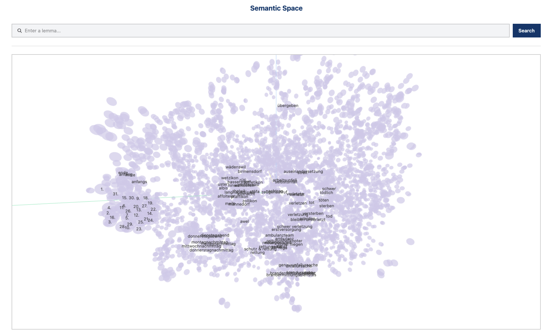
Fig. 10 Semantic space in the DE Demo Corpus.#
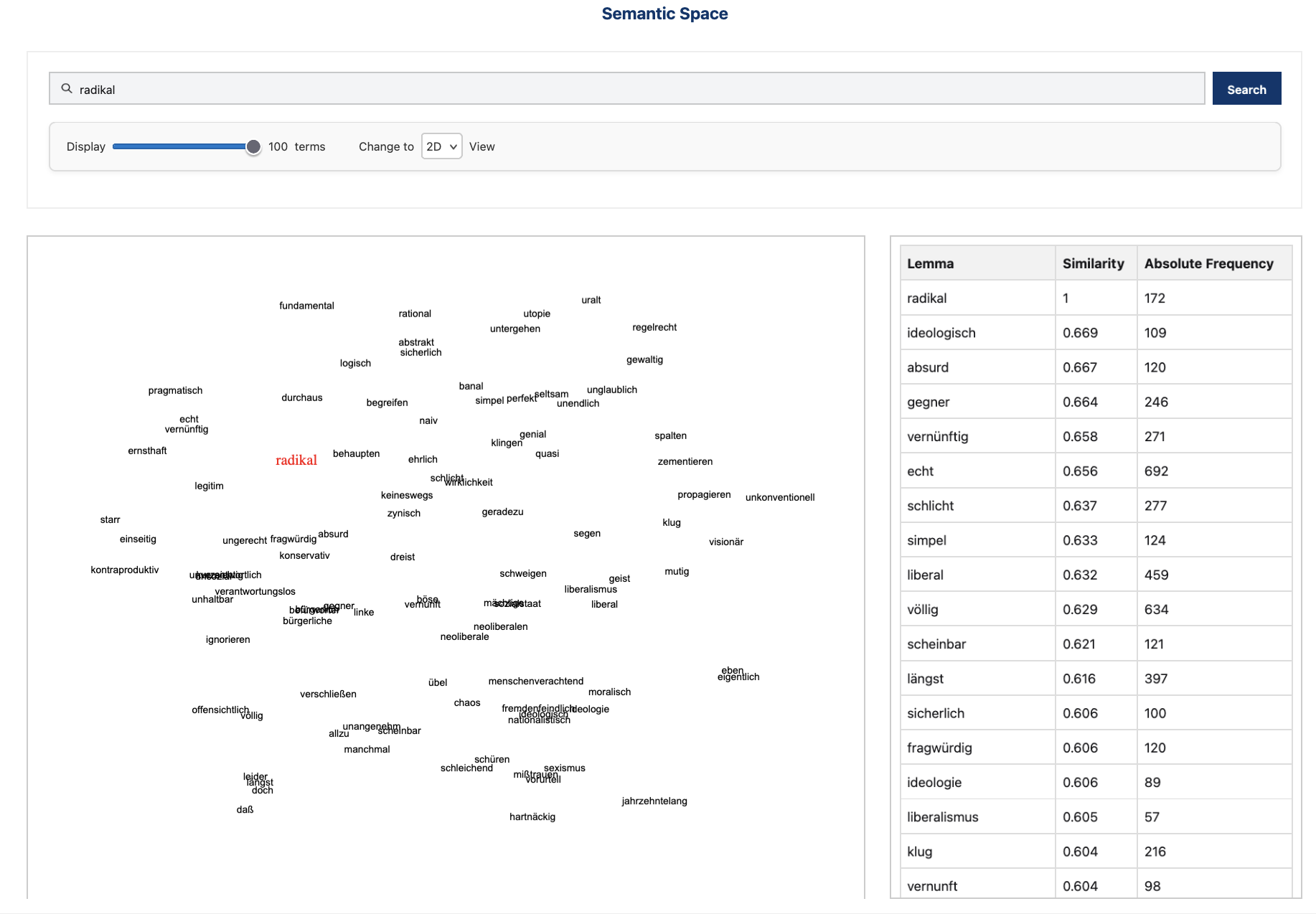
Fig. 11 Semantic neighbours for radikal (‘radical’) in the DE Demo Corpus.#
How the semantic space is calculated
Semantic spaces rest on the distributional hypothesis: words used in similar contexts tend to have similar meanings. If doctor and physician both appear alongside patient, hospital, and treatment, the model places them close together — without anyone telling it what either word means.
To learn this, the model reads through the corpus and records which lemmas occur near which others. Every lemma then gets a vector, a list of numbers describing the contexts it appears in, and lemmas with similar vectors count as similar. The similarity between two lemmas is reported as cosine similarity, running from 1 for near-identical contexts down to 0 for unrelated ones.
Because the models are built on lemmas, inflected forms are collapsed into a single entry.
Settings used on the platform
Algorithm |
word2vec (CBOW), via gensim |
Context window |
5 lemmas either side |
Vector size |
100 dimensions |
Minimum frequency |
5 occurrences |
Visualisation |
t-SNE with cosine distance, fixed random seed |
The diagrams compress 100 dimensions into two or three so they can be drawn, which loses information. They are also two separate projections: the corpus-wide diagram covers the 5,000 most frequent lemmas and is calculated once per model, while the neighbour diagram is calculated for each search and shows only your term and its 100 nearest neighbours.
Caution
Nearest neighbours are words used in similar contexts, which is not the same as words with similar meanings. Opposites are a common case: hot and cold, or war and peace, appear in almost identical contexts and often surface as close neighbours. Hyponyms, alternative spellings, and typos cluster for the same reason.
Treat the neighbour list as a starting point for interpretation rather than a result in itself, and check how the words are actually used — for example with Context of Words.
See also
For the potential of word embeddings in discourse analysis, see Bubenhofer et al. 2019. For the general principle behind word embeddings, we recommend Lenci 2018.